Abstract
Fast fourth-order linearized alternating direction implicit (ADI )and locally one-dimensional (LOD)schemes are presented to solve two-dimensional nonlinear riesz space fractional diffusion equations (RSFDEs). The proposed schemes employ the Crank-Nicolson method for temporal discretization,a quartic approximation for the Riesz derivative,and an explicit treatment for linearizing the nonlinear term. Through a rigorous discrete energy analysis,we derive explicit error estimates,proving that both schemes achieve second-order accuracy in time and fourth-order accuracy in space. The ADI and LOD methods are employed to decompose two-dimensional problems into a collection of symmetric positive definite (SPD)Toeplitz systems,for which the fast sine transform can be utilized to mitigate computational complexity. The computational treatment of these subsystems is further conducted using a preconditioned conjugate gradient (PCG )approach that leverages sine transforms. Theoretical analysis demonstrates that the preconditioned matrix can be decomposed into the identity matrix,a matrix of small norm,and a low-rank matrix. The effectiveness and efficiency of the scheme are validated through numerical examples.
0 Introduction
Considerable attention has been focused on space fractional differential equations(SFDEs)in recent decades due to their extensive applications in diverse fields,such as fluid mechanics[1],physics[2],and finance[3-4]. However,the nonlocality inherent in fractional calculus means that closed-form solutions to these equations are rarely attainable,making the development of robust numerical methods essential.
Consequently,numerous numerical schemes have been proposed for solving fractional diffusion equations[5-13]. To date,two principal methodologies have been widely adopted for the numerical approximation of Riesz fractional derivatives. The first approach,introduced by Ortigueira[ 14],is based on the fractional centered difference scheme. This method was later applied by Çelik and Duman[15]to riesz space fractional diffusion equations(RSFDEs),demonstrating that it achieves second-order convergence.The second major methodology originates from the work of Meerschaert and Dadjeran[5],who proposed a shifted Grünwald-Letnikov approximation for the Riemann-Liouville(RL)derivative. This foundation subsequently facilitated the development of the weighted shifted Grünwald-Letnikov difference(WSGD)scheme for solving RSFDEs[16]. Further advancing this line of research,Zhou et al.[17]constructed a quasi-compact discretization scheme with third-order accuracy. More recently,building on the WSGD approach,Hao et al.[18]introduced a higher-order scheme attaining fourth-order precision.
However,dense coefficient matrices are generated in the discretized systems because of the non-local nature of fractional derivatives,thereby imposing heavy computational and memory burdens on solving the resulting linear systems. With the development of numerical methods,several robust preconditioners have been proposed to tackle this issue in Toeplitz systems. For instance,Yu et al.[19]formulated preconditioned conjugate gradient(PCG)methods based on T. Chan[20]and R. Chan's[21]circulant preconditioners to address the challenges of solving Riesz distributed-order nonlinear SFDEs.Meanwhile,utilizing the approximate inverse preconditioning technique based on the inverse of R.Chan's[21]circulant matrix,Tang et al.[22]developed an efficient second-order numerical method for solving SFDEs with variable coefficients. The preconditioning approach incorporating the -preconditioner has emerged as a promising method for solving SFDEs[23-25].
When it comes to modeling and simulating multidimensional systems,the numerical discretization of partial differential equations,which is fundamental to the process,proves to be computationally expensive. By reducing multidimensional partial differential equations to a sequence of one-dimensional problems,alternating direction implicit(ADI)and locally one-dimensional(LOD)methods offer a simplified approach[26-30]. Recently,Tang and Huang[31]employed the ADI method to decompose the discretized linear system into multiple subsystems,which yielded first-order accuracy in space. They then combined the generalized minium residual(GMRES)method with the constructed large language model-augmented semantic digital twins(LSDTs)-preconditioner to solve these subsystems. Chen et al.[32]developed a second-order LOD multigrid method for multidimensional RSFDEs. Combining the backward differentiation formula(BDF)method with a fourth-order fractional compact operator,Hu and Cao[33]constructed a high-accuracy ADI scheme for2D nonlinear RSFDEs. However,the development of a fast algorithm was not addressed. The scarcity of high-order fast algorithms based on the ADI and LOD methods for multidimensional RSFDEs has motivated our research in this direction.
In this study,we investigate the following 2D nonlinear RSFDEs:
(1)
where p and φ are sufficiently smooth in their respective domains. β,γ ∈(1,2)and Ω=(0,L1)×(0,L2),L1,L2and T are positive constants. Kβ,Kγ>0,f(u)is a continuous function and satisfies the Lipschitz condition. Moreover, and denote the Riesz fractional derivative[23,25].
In this study,fourth-order linearized ADI and LOD schemes are proposed to solve 2D nonlinear problem(1). Both proposed schemes employ the Crank-Nicolson method for temporal discretization and a fourth-order approximation[18]for the Riesz derivative,along with explicit linearization of the nonlinear terms. Both schemes are proven to achieve second-order temporal accuracy and fourth-order spatial accuracy,as established through explicit error estimates derived from a discrete energy analysis. The ADI and LOD methods are employed to decompose two-dimensional problems into a collection of symmetric positive definite(SPD)Toeplitz systems,for which the fast sine transform can be utilized to mitigate computational complexity. The solution of these subsystems is achieved through the application of the PCG method preconditioned by the -matrix approximation. In addition,theoretical analysis confirms that the τ-preconditioner matrix exhibits eigenvalues tightly clustered around unity,while numerical results substantiate the extended τ-preconditioner's remarkable efficacy in accelerating convergence for two-dimensional problems.
The study is structured as follows. In Section 1,linearized fourth-order ADI and LOD schemes are developed for the nonlinear RSFDEs. The PCG method with a -preconditioner is presented in Section 2 to accelerate the solution of discrete linear systems,and the spectral characteristics of the preconditioned matrices are analyzed. In Section 3,numerical examples are conducted to demonstrate the convergence behavior and computational efficiency of the fast numerical schemes incorporating preconditioners. A summary of key findings is offered in Section 4.
1 Linearized Numerical Scheme
1.1 Derivation of the Numerical Scheme
Take positive integers M1,M2 and N. Denote Δx=, and ,Let,and },xi=,yj= iΔy(j ∈ [[0,M2+1]]),tk= kΔt (k ∈ [[0,N]]),{(xi,yi)| i ∈[[0,M1+ 1]],j ∈ [[0,M2+ 1]]},,,ω={(i,j)∣(xi,yj)∈ },={(i,j)∣(xi,yj)∈},= ω∪,ΩΔt={t k ∣0≤k ≤ N},Vh={u ∣ u={ui,j ∣(i,j)∈ }}.
Given any discrete function u ∈ Vh,we define
,
where
Define
Let
where k ≥ 2,.
Lemma 1[18] Assuming α ∈ (1,2) , the coefficients satisfy
Let
Define the following difference operator:
Lemma 2[34] For any u(x,y,·) ∈ C3[0,T] ,we have
Denote
where F(k)is represented as the Fourier transformation of f(t).
Lemma 3[18] Let u(·,y,t) ∈( ℝ) , and u(x,·,t) ∈ ( ℝ) , we have
Lemma 4 Let f(u) ∈ C2(R) , then we have
Proof: By employing a Taylor series expansion,the correctness of the formula can be directly validated.
Building upon the foregoing lemmas,we now proceed to derive high-order numerical schemes for solving problem(1),under the assumption that the solution u(x,y,t)adheres to the conditions stipulated in Lemmas 2 and 3. Considering the main equation in problem(1)at(xi,yj,tk),and averaging two adjacent time layers,we have
(2)
Applying to Eq.(2)and using Lemmas 2-4,we have
(3)
where ,and
Adding to both sides of Eq.(3)gives
(4)
where
(5)
By omitting the small terms in Eq.(4)and substituting the exact solution with an approximated solution ,the following linearized numerical scheme for solving problem(1)is obtained
(6)
where .
Multiplying both sides of the main equation in Eq.(6)by Δt yields the resulting form
By introducing the intermediate variable ,we have the following linearized ADI scheme:
(7)
We now develop a linearized LOD scheme.Adding small term
to both sides of Eq.(4)yields
(8)
where
(9)
By omitting the small terms in Eq.(8)and substituting the exact solution with an approximated solution,the following linearized numerical scheme for solving problem(1)is obtained:
(10)
We multiply both sides of the main equation in Eq.(10)by Δt and reformulate it as
By introducing the intermediate variable ,we have the following linearized LOD scheme:
(11)
Let
and we assume that and share a common upper bound,i.e.,
(12)
where μ is a real number.
Let
(13)
where(M,α)=(M1,β)or(M2,γ).
Define
(14)
where
(15)
where(M,α)=(M1 ,β)or(M2,γ).
Clearly,and ±are the symmetric Toeplitz(ST)matrices.
We define the following M-order symmetric tridiagonal matrices:
where(M,α)=(M1,β)or(M2 ,γ).
Define
We then derive the matrix form of the linearized ADI scheme as follows:
(16)
Let
where
Then,we arrive at the following matrix form of the linearized LOD scheme:
(17)
1.2 Error Estimate
Let ;if(i,j)∈ ∂ω,ui,j= 0}.Given any discrete functions u, v ∈ ,we define(u,v)= ΔxΔy,‖u‖=
Sinceandare positive definite and self-adjoint,we have=and= [18].
Lemma 5[18] For any grid function u ∈, we have
According to the definitions of and ,it is straightforward to show that both- and- are symmetric positive definite operators. Therefore,there exist fractional symmetric positive definite difference operators Λx and Λy such that the following conclusions hold[18]:
Lemma 6 For any grid function u ∈ , we have
Proof: By Lemma 5, we get
The proof is completed.
Lemma 7[30] Assume that {} and {} are nonnegative sequences, and that the sequence {}satisfies
Then it holds that
We begin with an analysis of the stability and convergence of the linearized ADI scheme in Eq.(7).Let ,by subtracting the master equation in Eq.(6)from Eq.(4),we get
(18)
Theorem 1 Let be the solution of Eq.(18)and Δt < 1 / (18(L +)) , we have
where c is a constant independent of Δx,Δy and Δt,and L is the Lipschitz constant of the function f(u).
Proof: Forming the inner product of Eq.(18)with gives
(19)
Let =,=,we have
(20a)
(20b)
When n ≥ 1,an application of Lemma 5,coupled with the Lipschitz condition and the Schwarz inequality,leads to
(21)
By the same reasoning,we obtain
(22)
Inserting Eq.(20)and inequalities(21)-(22)into Eq.(19),and using Lemma 6,yields
Therefore,for all n ≥ 2,
(23)
Upon taking the inner product of Eq.(18)with for the case n= 0,and noting the identity -= 0,we establish that
(24)
Using Eq.(20)and Lemma 6,we obtain
(25)
It follows from Lemma 5,the definition of E1,and inequality(25)that
(26)
Substituting inequality(26)into(25),we obtain
(27)
Inserting inequality(27)into(23)yields
Using Lemma 5 and the definition of ,we get
When Δt < 1/(18(L+)),
By Lemma 7,we get
From Eqs.(5)and(26),we obtain the required result immediately.
Remark 1 The stability of the linearized ADI scheme (7) can be readily established in a similar manner.
In what follows,we focus exclusively on the error estimates of the LOD scheme for linear equations. We consider the linear version of problem(1),which is formulated by discarding the nonlinear term. For this linear equation,the compact LOD scheme is given by
(28)
Let ,by subtracting the master equation in Eq.(28)from Eq.(8)and neglecting the nonlinear terms,we get
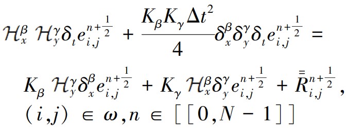
(29)
where = O(Δt2+ Δx4+ Δy4),n ≥ 0.
Theorem 2 Let be the solution of Eq.(29)and Δt <, we have
where c is a constant independent of Δx,Δy and Δt.
Proof: By forming the inner product of Eq.(29)with , we get
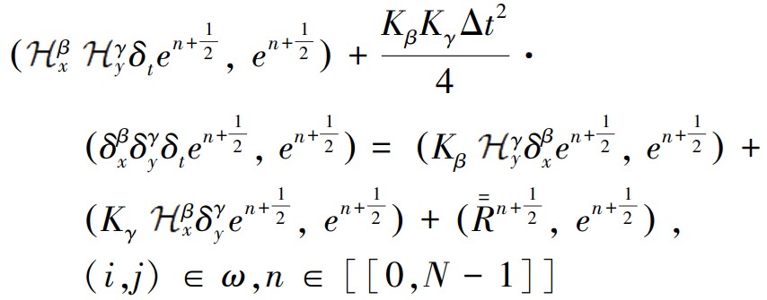
Let = ,=. By Lemma 6,we obtain
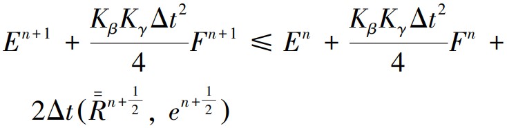
Therefore,for all n ≥ 1,
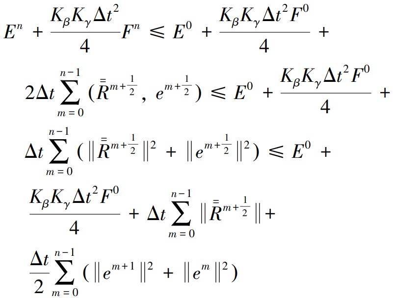
By Lemma 5 and the definitions of and ,we get
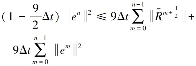
When Δt< 1/ 9,

By Lemma 7,we get

From the definition of ,the needed result follows immediately.
,the needed result follows immediately.
Remark 2 The stability of the LOD scheme(28) can be easily proved through an analogous approach.
2 PCG Method
The CG method is a well-known and efficient technique for solving linear systems(16)and(17).However,experiments indicate that the coefficient matrix has a widely distributed eigenvalue spectrum,which significantly degrades the convergence rate of the standard CG method. To address this issue,this section introduces a PCG approach that utilizes theτ-preconditioner to accelerate convergence for these systems. Next,we introduce a τ-preconditioner derived from the sine transform.
For any Toeplitz matrix
the generating function of can be defined as
where p(θ)is in the Wiener class if and only if [25]. In particular,if ,then is symmetric,and we denote it as . Let be a Hankel matrix with antidiagonal entries
Then,the -matrix ()can be described by ()= -[25]. Hence,we propose the -preconditioners of the linear systems(16)and(17)as
(30)
The dominant computational overhead of PCG when applied to linear systems(16)and(17)arises from evaluating and . Leveraging the Toeplitz property of and the diagonalizability of,these matrix-vector multiplications achieve an optimal complexity of O(Mlog(M))(M1=M2= M)[25].
Lemma 8[35] If is a ST matrix with the first column being . Then, the eigenvalues of τ() can be given by
Lemma 9 τ() in Eq. ( 30) is SPD, and,(M,α) = (M1 ,β) or (M2 ,γ).
Proof: Since is an ST matrix and τ() is defined by Eq. ( 30 ), it follows that τ() is a symmetric matrix. We apply Lemma 8 and Lemma 1while taking into account < 0 and to obtain
Therefore,the matrix τ()is SPD,and we can further obtain that
This completes the proof.
Lemma 10 Let be defined by Eq. ( 15).Under the assumption (12), the generating functions of ( (M,α) = (M1 ,β) or (M2 ,γ) ) are in the Wiener class.
Proof: Applying Lemma 1, and noting that , we deduce that
This completes the proof.
Lemma 11[35] If the generating function of is in the Wiener class, then for any ε > 0,there exists > 0 such that for all M > ,
where and rank.
Theorem 3 Let and τ() be defined by Eqs. ( 14 ) and ( 30 ), respectively. Under the assumption ( 12), and then for any ε > 0, there exists > 0 such that for all M > ,
where and rank(VM)≤ ,(M,α)=(M1,β)or(M2,γ).
Proof: From the definition of and Lemmas10-11, we get
(31)
where
(32)
Multiplying both sides of Eq.(31)by,we have
where and .
Applying Lemma 9 and inequality(32),we have
This completes the proof.
According to the Weyl's theorem,Theorem 3indicates the spectrum of is clustered around 1[36]. This typically leads to a fast convergence rate for the PCG method in solving linear systems(16)and(17)[24-25,36].
3 Numerical Results
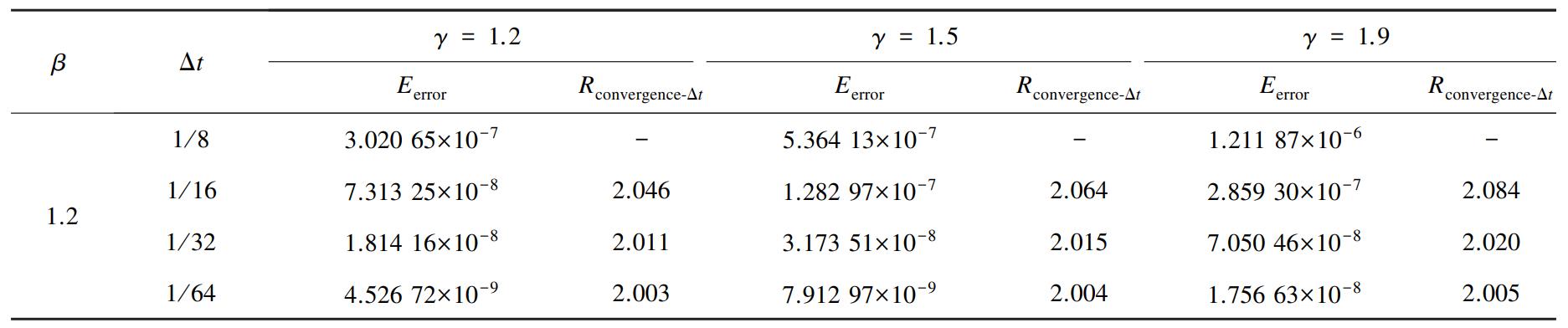
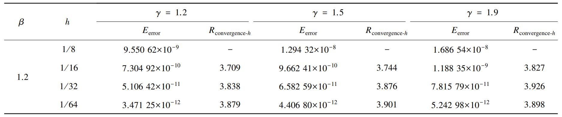
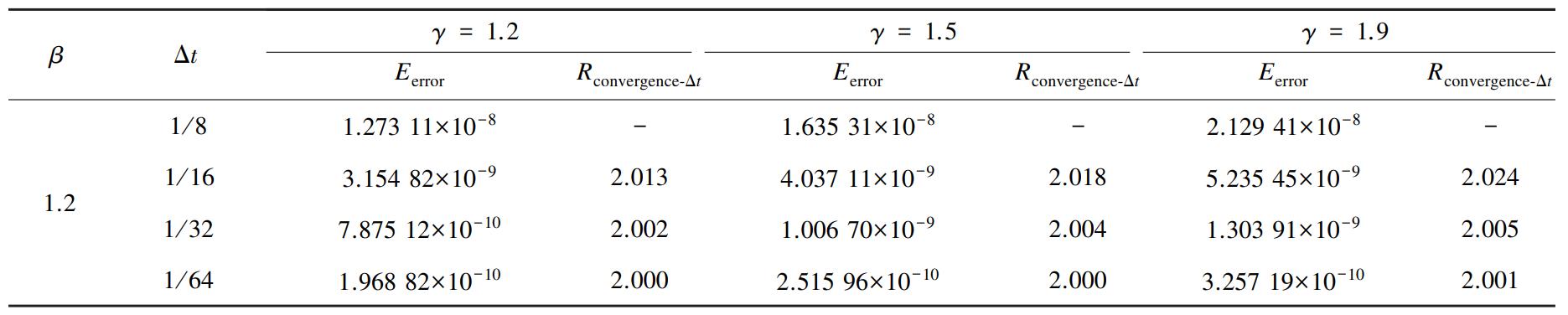
A series of numerical tests are performed to evaluate the method's effectiveness. We set the stopping criterion to be < 10-7.As shown in Tables 1-8,the acronyms “CG-LOD”and “CG-ADI” denote the base CG method for the linearized LOD and ADI schemes,respectively.“PCG-LOD(τ)” and “ PCG-ADI(τ)” represent our proposed PCG method with the τ-preconditioner.“ PCG-LOD(S/ T)” and “ PCG-ADI(S/ T)”indicate the PCG methods with Strang's[37]and T.Chan's[20]circulant preconditioners,respectively.“Time(s)” denotes the total CPU time in seconds.“ Iter ” represents the average number of iterations across all time steps for solving linear systems in both directions. Let Δx= Δy= h. Define
Table
1
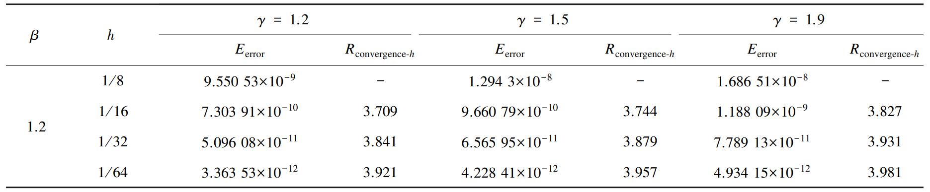
Temporal errors and convergence rates of the LOD scheme (11)with h= 1/ 200
Table
2
Spatial errors and convergence rates of the LOD scheme (11)with Δt= 1/ 10 000
Table
3
Temporal errors and convergence rates of the ADI scheme (7)with h= 1/ 200
Table
4
Spatial errors and convergence rates of the ADI scheme (7)with Δt= 1/ 10 000
Example 1 Consider the problem(1)with Kβ= Kγ= 1,L1= L2= T= 1,f(u)= sin(u),
and
The exact solution is
Tables 1-4 describe the numerical outcomes for solving Example 1,showing the errors and convergence rates for the linearized ADI scheme(7)and LOD scheme(11). It can be seen that both schemes achieve second-order temporal convergence and fourth-order spatial convergence.
Table
5
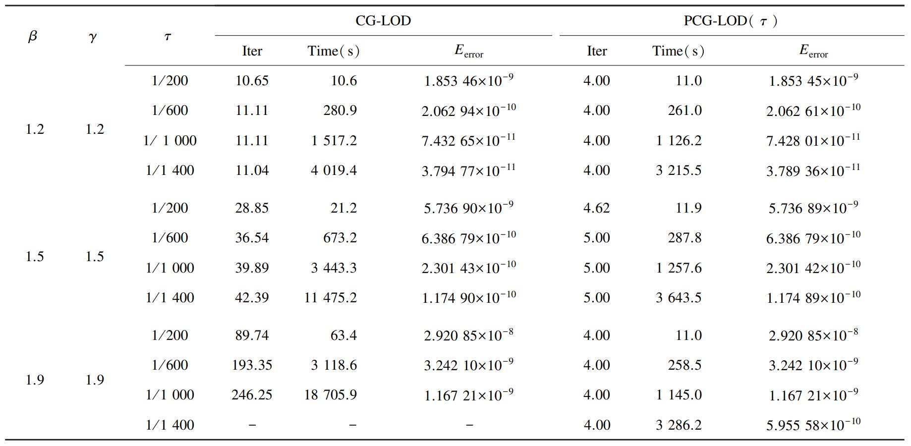
Comparisons of PCG-LOD(τ)method and the CG-LOD method with Δt= 2h
Table
6
Comparisons of PCG-ADI(τ)method and the CG-ADI method with Δt= 2h
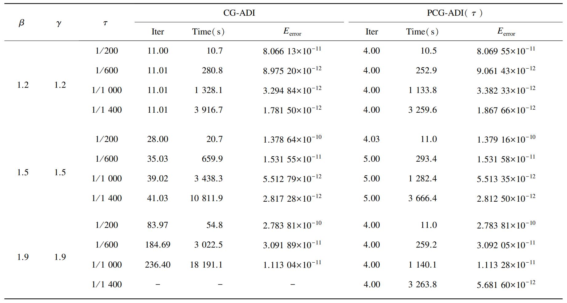
In Tables 5-6,we compare the performance of our PCG-LOD(τ)and PCG-ADI(τ)methods with those of the CG-LOD and CG-ADI methods. It is evident that PCG-LOD(τ)and PCG-ADI(τ)achieve both a lower iteration count and reduced computational time. For instance,when β= γ= 1.9,h= 1/ 1 000,the CG-LOD method achieves an accuracy of 1.167 21×10-9at the cost of an average of246. 25 iterations and 18 705.9 s. In contrast,PCG-LOD(τ)achieves the same precision with only 4.00 iterations on average and a computation time of1 145.0 s. The results demonstrate that the proposed methods markedly enhance computational efficiency.
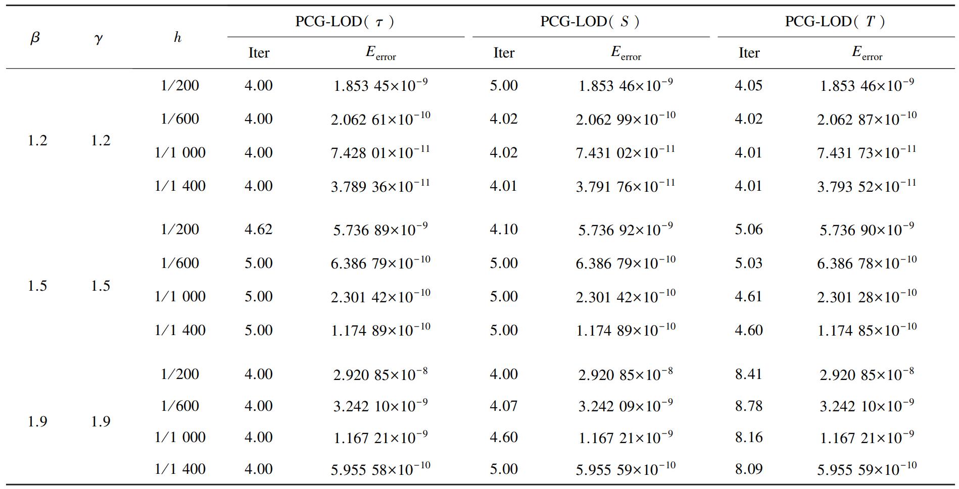
Existing circulant preconditioners have been developed for solving the linear systems(16)and(17)with the ST coefficient matrices[20,37]. As indicated in Tables 7-8,our PCG-LOD(τ)and PCG-ADI(τ)methods outperform the existing methods in terms of average iteration count,including PCG-LOD(S/ T )and PCG-ADI( S/ T).
The spectra of several preconditioned matrices are presented in Figs. 1 and 2. As clearly shown,matricesand exhibit significantly greater spectral concentration compared with matrices,,and. The average iteration numbers for various preconditioning methods,presented in Tables 7-8,lend further support to this conclusion.
Table
7
Performance of different PCG methods with Δt= 2h
Table
8
Performance of different PCG methods with Δt= 2h
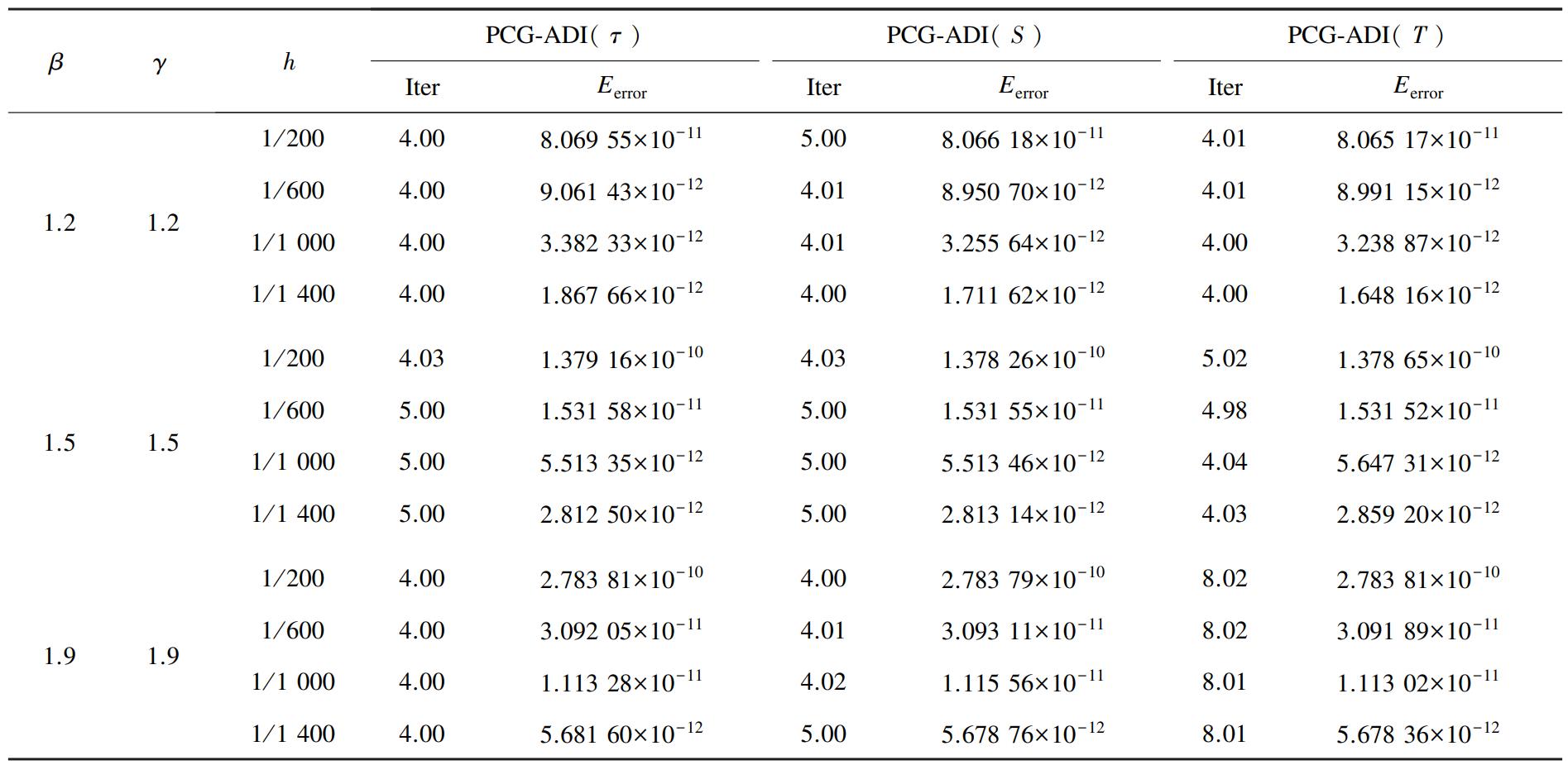
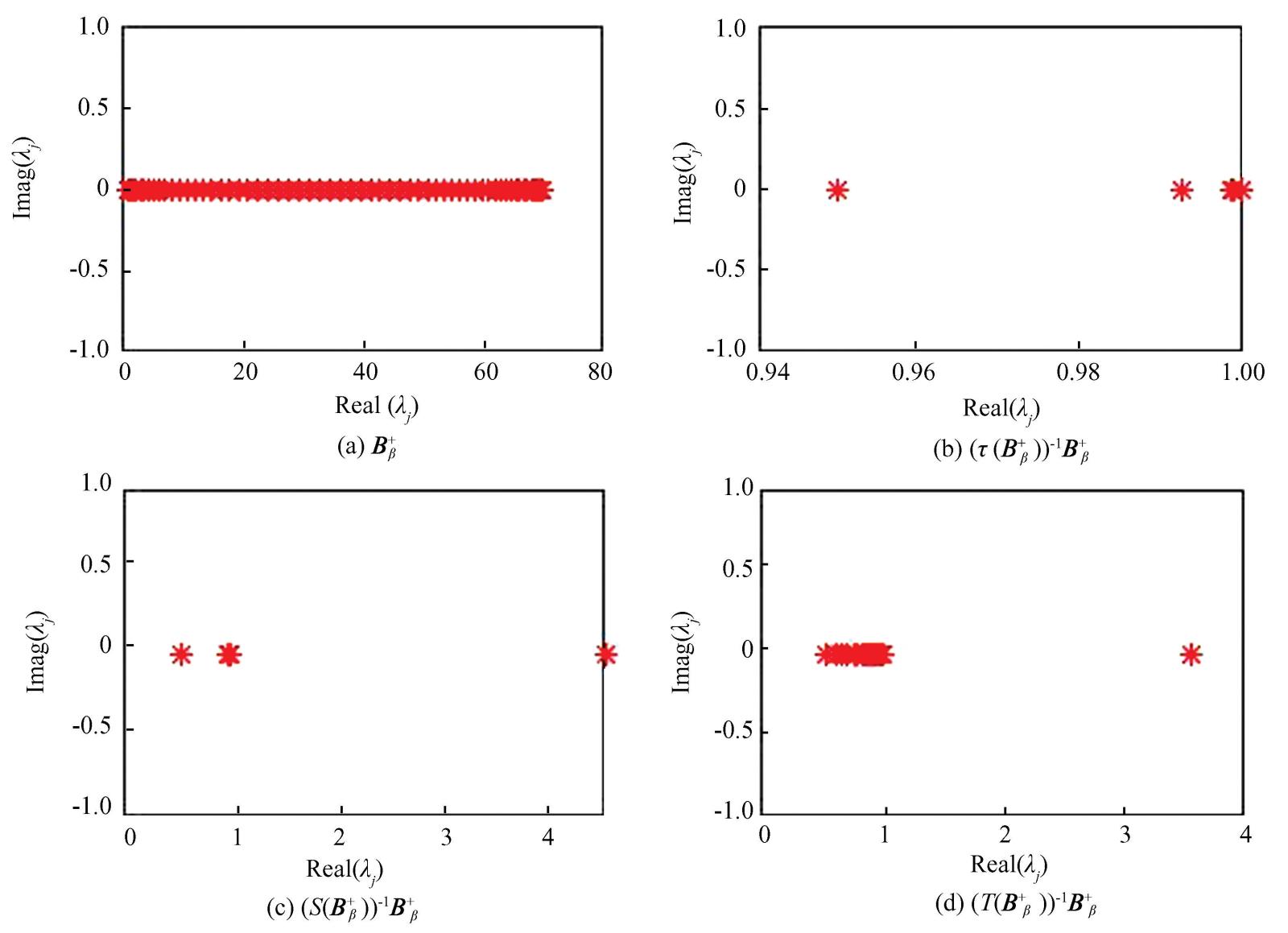
Fig.
1
The spectrum of ,, and with h= Δt= 1/ 26 and β=γ= 1.9 for Example 1
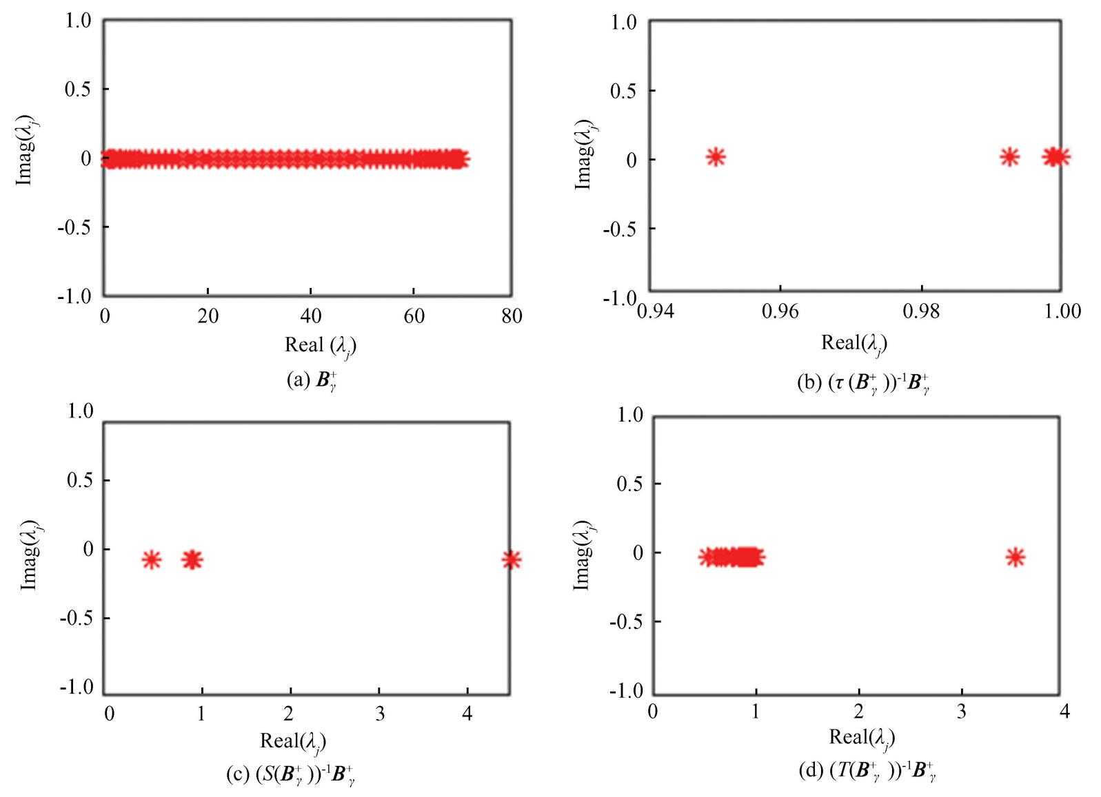
Fig.
2
The spectrum of ,, and with h= Δt= 1/ 26and β=γ= 1.9 for Example 1
4 Conclusions
Fourth-order linearized ADI and LOD methods are derived herein to solve 2D nonlinear RSFDEs numerically. Discrete energy analysis provides explicit error estimates that establish the second-order temporal and fourth-order spatial accuracy of both schemes.Moreover,the PCG method,which incorporates a τ-preconditioner,is employed to solve these discrete linear systems. It has been theoretically proved that the preconditioned matrix can be decomposed into the sum of an identity matrix,a small-norm matrix,and a low-rank matrix. As demonstrated by numerical tests,both methods with τ-preconditioner outperform existing methods in both iteration efficiency and computational cost. Furthermore,preliminary evidence suggests that the proposed τ-preconditioner may also be applicable to the ADI scheme developed by Hu and Cao[33],which constitutes a pertinent subject for our further investigation.
Conflicts of Interest
The authors declare no potential conflicts of interest.
