Abstract
As connected and automated vehicles (CAVs)and connected human-driven vehicles (CHVs)show a considerable difference in efficiency and control,currently existing measures that separate the mixed traffic at intersections often depend on CAV penetration. This dependency limits the applicability of these methods. This study presents an efficient separation control method at a low level of CAV penetration to overcome this limitation. The main idea of the method is to use pre-signals to separate upstream CAVs from CHVs and then guide CAVs to dedicated lanes.In this scenario,at CAV penetration below 30%,start-up losses during the green phase can be reduced. Based on this configuration,a joint optimization model is proposed that couples vehicle trajectories with traffic signals while taking into consideration the constraints between the pre-signal and the main signal. The aim is to minimize average vehicle delay,while the particle swarm optimization algorithm is utilized to solve the model. According to simulations,the average vehicle delay is decreased by 28.27% compared to a first-come-first-served design and by 19.4% compared to a design of phase continuous tandem intersections. The CAV penetration rate,as well as the queue area length,has a significant influence on the control effectiveness. Researchers identify an optimal design value of a CAV penetration rate below 30%and a queue area length of 45 m.
0 Introduction
Connected human-driven vehicles(CHVs)play an essential role in the use of human-driven vehicles,which further facilitates the transition from human to autonomous driving. Increased CHV penetration rates and increased driver compliance will greatly contribute to traffic stability[1]. At the same time,the penetration rate of connected and automated vehicles(CAVs)is also important. Mixed traffic environments directly affect the overall efficiency and performance in terms of energy consumption[2]. The CAV penetration rate determines how effective the control strategies are. In the case of low penetration rates,an adaptive traffic signal control system using model predictive control(MPC)[3]and deep reinforcement learning(DRL)[4]has been found to be effective. These systems can optimize the interaction between CAVs and CHVs.Through this optimization,they can reduce the vehicles' travel time and fuel consumption. On the contrary,under high-penetration conditions,adopting a dedicated intersection management strategy that separates CAVs from CHVs will significantly improve the efficiency of mixed traffic flow[5].
Due to significant differences in response speed,decision logic,and behavioral patterns between CAVs and CHVs,intersection management is complex.Previous research has developed intersection capacity models for mixed flows of autonomous and human-driven vehicles[6]. There are also studies that can optimize management strategies by setting up CAV-dedicated lanes[7]. The results indicate a positive correlation between CAV penetration rate and mixed traffic capacity. In addition,infrastructure-assisted collaborative driving has also brought new ideas for optimizing control at signalized intersections. The optimization model that combines CAV trajectories with traffic signals can significantly reduce average delay and fuel consumption,highlighting the potential of intelligent intersection management[8].
Intersections are a key bottleneck in transportation networks and have long been a focus of traffic control research. As technology progresses,regulations and policies evolve,and mixed traffic flow of human-driven vehicles and autonomous vehicles will continue to be the main form of flow at intersections until full automation occurs. Thus,the development of more advanced intersection control methods is needed[9]. As a result,many innovative signal-control strategies have been proposed for mixed traffic conditions. One approach could be to add a “white phase” to the CAV passage time[10]. Another study combined all red control with a flexible signal timing method(FMAA)for mitigating conflicting traffic at isolated intersections[11].Additional innovations involve enhancing traffic smoothness utilizing stochastic distribution control rationale[12]and employing coordination graphs to regulate the control of traffic signals[13]. There is also an intelligent fuzzy control system design based on symmetry theory[14]. In addition to improving traffic efficiency,the research uses VSP models to measure the effect of signal control on emissions[15]. Due to the continuous and changing traffic flow characteristics,the multi-agent system(MAS)is gaining widespread acceptance in intersection management[16]. The safety and efficiency issues that arise from mixed traffic are constantly being addressed through new methods. For instance,the robot vehicle(RV)[17]control model and the multi-user traffic assignment model based on variational inequalities[18]are exemplary. Moreover,urban traffic management has been introduced to macro-micro comprehensive control strategies. An example is the dynamic zone sowing algorithm(DZSA),which was designed to ease congestion in cities[19].
Along with these types of controls,the use of pre-signal control is another useful measure. The priority of buses was initially raised using pre-signal control. The use of a pre-parking position allows buses that arrive at red lights to queue ahead of ordinary vehicles. This allows buses to gain priority passage when the light turns green. Over the years,this concept has been expanded and implemented in various unconventional intersection designs. For example,it is utilized at tandem intersections,continuous flow intersections,as well as U-turn intersections to improve the regulation of turning and straight traffic. Research has shown that combining pre-signals with queuing areas can increase the capacity of mixed traffic flow[20]. Applications also include signal timing techniques that use reversible lanes for space reuse[21-22]. We use pre-signals to help intersections in a series work together with their signals and functions[23-25]. Through simulation and mathematical modeling of heterogeneous traffic environments,it has been shown that the cooperative driving strategy of CAVs and CHVs based on a pre-parking route offers significant advantages. These attributes can increase traffic capacity and lower energy consumption[26]. Another study may focus on the resolution of conflicts between motor vehicles and non-motor vehicles[27]and on the optimal utilization of lane resources[28]. Despite the progress made by these methods,most current research is still based on the assumption of homogeneous transportation. The new intersection control paradigm has not yet fully utilized the potential of heterogeneous traffic flows.
According to studies,saturation flow in mixed lanes is more strongly affected by the penetration rate of CAVs[29]. When the penetration rate exceeds the threshold,there are substantial benefits to separating CAV from CHV operations. Currently,the primary means of effecting this separation is through CAV-dedicated lanes. Rey and Levin[30] were the first to introduce this concept into intersections and research in this direction continued thereafter. As an example,Jiang and Shang[31]proposed a dynamic allocation method for CAV-dedicated lanes. The purpose of this method is to address the problem of uneven lane utilization due to variations in penetration rate. To further increase the utilization potential of CAV-dedicated lanes,Ma et al.[32]proposed an optimization control method for left-turn and through CAVs to share the same lane. But the shared lane is still statically configured. Due to this shortcoming,Hu et al.[33]established a configuration method for CAV-shared lanes through a conversion index. By using this method to determine whether the timing for shared lanes is dynamically responsive to changes in traffic demand,utilization can be enhanced. Despite being optimistic about the establishment of CAV-dedicated lanes at intersections,these studies point to a limitation in their applicability:dedicated lanes are not useful at lower CAV penetration rates. When there is low penetration,dedicated lanes can lead to disproportionality in the allocation of resources,thus affecting control and causing disarray.
To address the above issues,this study proposes a separation control method for mixed traffic that combines pre-signals with CAV-dedicated lanes. The main contributions are as follows:
1)A novel separation control framework for human-machine hybrid driving is introduced to address the impact of low CAV penetration on CAV-dedicated lane settings,utilizing pre-signals and CAV-dedicated lanes;
2)A trajectory signal joint optimization model is developed to minimize the average delay by utilizing the high maneuverability of CAV and combining the main and pre-signals with vehicle lane changing and trajectory optimization;
3)A comprehensive sensitivity analysis is performed to delineate the boundary conditions of the proposed method,including CAV penetration rate and queue length,to verify their significant impact on the control effectiveness of the optimization method.
The structure of the article is as follows. In Section 1,the concept of traffic flow separation is introduced through human-machine hybrid driving.The mathematical model of the method and the solution algorithm are developed in Section 2. Section3 contains the numerical experiments used to evaluate the proposed algorithm. Section 4 contains the analysis of the experiments. Section 5 provides a summary of findings and recommendations for future work.
1 Problem Statement
CAVs and CHVs differ significantly in maneuverability and controllability. Roadways are crowded with all kinds of vehicles,which tech-savvy CAVs cannot fully take advantage of. This leads to improper utilization of road space and time. For this purpose,researchers have developed many optimization strategies. These strategies manage traffic at junctions with different types of vehicles. The primary objective is to improve traffic efficiency and reduce energy consumption.Alternatively,they seek to enhance driver comfort and maintain road safety at the same time.
At low CAV penetration rates,both domestic and international researchers have investigated methods for integrating CAVs and CHVs into entrance lanes to optimize traffic flow. Although some studies proposed using CAVs to lead CHVs to form queues as an optimization strategy[34],the lack of controllability of CHVs diminishes the effectiveness of these methods and introduces potential safety risks. Moreover,the mixed operation of CAVs and CHVs fails to exploit the high maneuverability and controllability advantages of CAVs. To address these challenges,this study proposes a separation control method for human-machine mixed driving traffic flow(SCM-MT)based on pre-signals and CAV-dedicated lanes at intersections. The SCM-MT aims to overcome the limitations imposed by low CAV penetration rates on the implementation of CAV-dedicated lanes,as illustrated in Fig. 1. Furthermore,the penetration rate of CAV set in this article is lower than 30%.
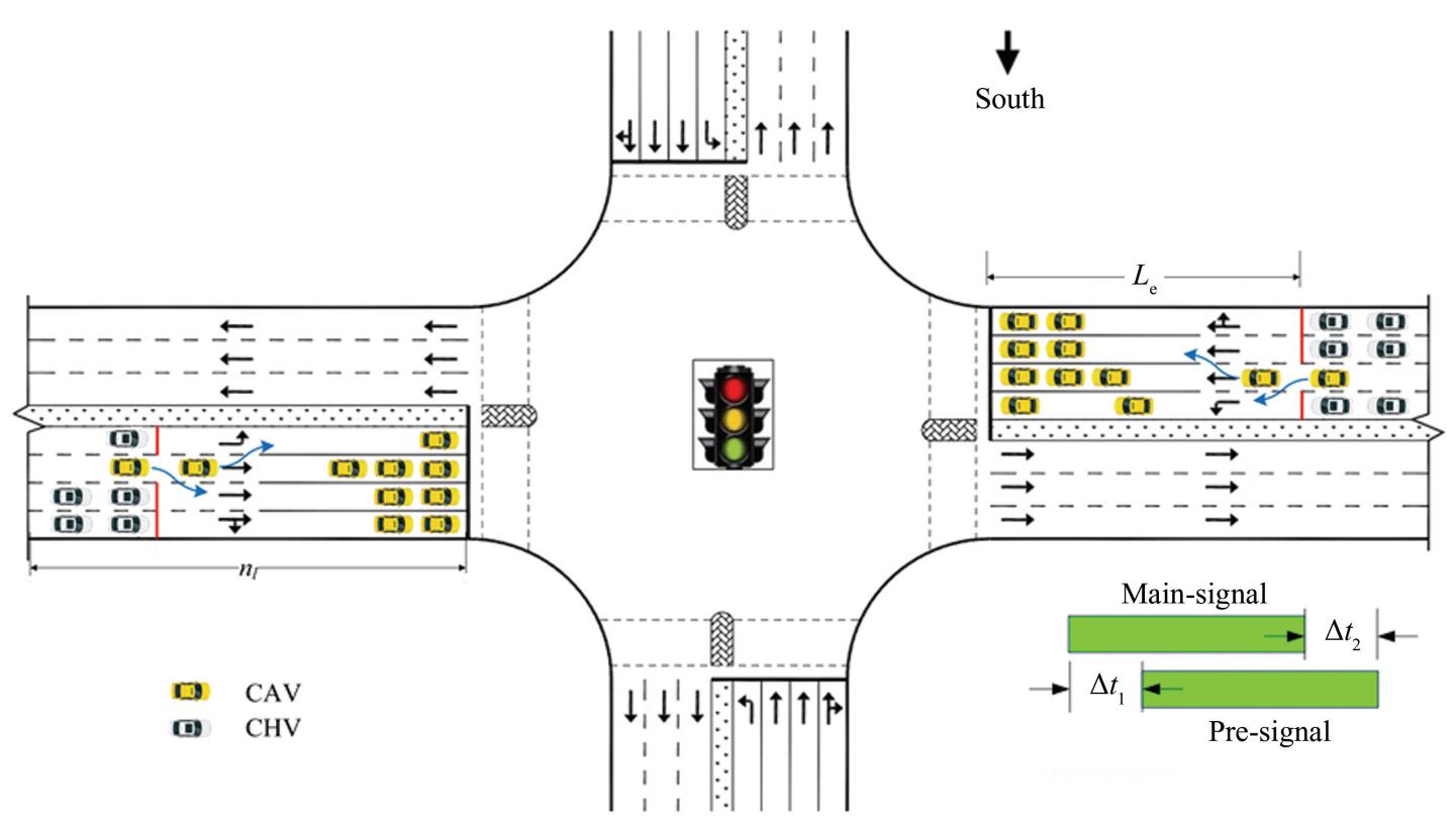
Fig.
1
Schematic of SCM-MT
The SCM-MT designates the through lane adjacent to the left-turn lane as a CAV-dedicated lane.Additionally,a second stop line and traffic lights were implemented in all lanes except the CAV-dedicated lane. The area between the main stop line and the second stop line serves as the CAV lane-changing and queuing zone. Pre-signals and CAV-dedicated lanes were used to separate CAVs from CHVs in the approach lanes of the intersection. During the red time of the pre-signal,the left-turn CHVs and through-CHVs queued up after the second stop line.Meanwhile,left-turn and through-CAVs utilize a CAV-dedicated lane to bypass the queue,proceeding directly to the prominent stop line and queuing in their respective designated areas. During the green signal phase of the pre-signal,the left-turn CHVs and left-turn CAVs queued behind the second stop line and proceeded through the left-turn lane in a first-come,first-served order. Through-CAVs and through-CHVs can temporarily share a CAV-dedicated lane,thereby improving their utilization efficiency. SCM-MT differs from traditional bus pre-signal methods in that the CAV-dedicated lane can accommodate both left-turning and through-CAVs during the red signal phase. Additionally,unlike tandem intersections,the functional assignments of the lanes in front of and behind the second stop line remain fixed,such as exclusive lanes for left turns or through movements.
Let 𝐿 represent the set of all lane groups at the intersection,𝐵𝑙 denote the set of all lanes within lane group 𝑙,and 𝐼𝑏𝑙 represent the set of all vehicles on lane 𝑏 ∈ 𝐵 within lane group 𝑙∈ 𝐿. If a CHV enters the communication range of an intersection,its entry time is recorded as 𝑡 𝑗𝑏𝑙. If the CAV must execute a lane change in the CAV-dedicated lane,its entry time is initially recorded as 𝑡 𝑛𝑎. After completing the lane change and entering a new lane,the entry time is updated and recorded as 𝑡 𝑖𝑏𝑙.
2 Optimization Methods
2.1 Model Construction
2.1.1 Objective function
The following optimization objective function is established to minimize the average delay of vehicles at intersections:
(1)
(2)
(3)
(4)
(5)
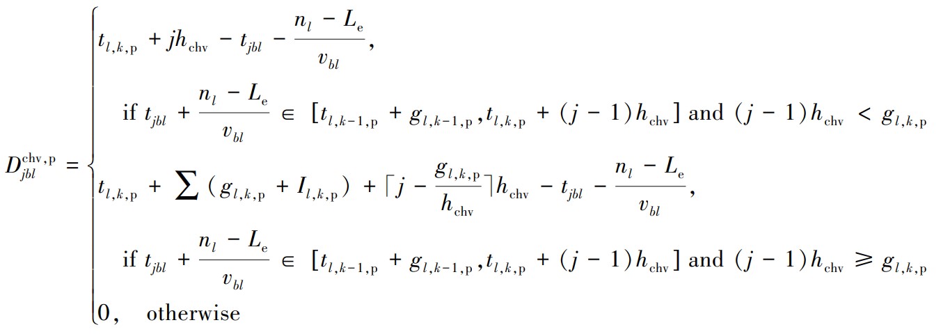
In these equations, represents the average delay for all vehicles at an intersection. refers to the delay encountered by the ith CAV on lane b within lane group 𝑙,while represents the delay experienced by the 𝑗th CHV in the same lane. The total number of CAVs traveling on lane 𝑏 in lane group 𝑙 is denoted by ,whereas represents the number of CHVs. represents the moments when the primary signal for lane group 𝑙 switches to green during the kth signal cycle. Meanwhile,𝜏ₐ,the start-up loss time for CAVs,captures the additional delay incurred during acceleration from a stationary state,and ℎcav signifies the saturated headway of CAVs. The distance between the entry point of a vehicle,the communication boundary of the intersection,and the main stop line is given by 𝑛𝑙,whereas 𝐿e specifies the length of the segment between the second and main stop lines. Furthermore,𝑣bl reflects the average speed of the vehicles in lane group 𝑏. The pre-signal green-time activation periods for lane group 𝑙 during the kth cycle are denoted as 𝑡 𝑙,𝑘,p. The saturated headway of the CHVs,ℎchv,describes the time interval between two consecutive CHVs passing through a given point under ideal traffic conditions. Additionally,𝑡 𝑗𝑏𝑙 marks the exact time at which the 𝑗th CHV in lane 𝑏 enters the communication boundary of the main signal. The pre-signal green time for lane group 𝑙 in the kth cycle is captured by 𝑔𝑙,𝑘,p,whereas 𝐼𝑙,𝑘,p denotes the pre-signal green interval during the same cycle. Finally,𝜏ℎ reflects the start-up loss time attributed to the CHVs.
Eq.(1)represents the total delay of connected vehicles,with the first term being the average delay of CAV vehicles in the queue area,the second term being the average delay of CHV vehicles in the CAV dedicated lane,and the third term being the average delay of CAV vehicles in the CAV dedicated lane.Eq.(2)defines how to calculate the delay for CAVs at the main signal. The delay equals the departure time(first three terms)minus the entry time at the communication boundary(fourth term). It also subtracts the expected travel time from the boundary to the main stop line(fifth term).
For CHVs,Eq.(3)defines the total delay. This delay includes two parts:the main signal-related delay and the pre-signal-related delay. Eq.(4)specifically calculates the main signal delay of CHVs. Eq.(5)further refines the three specific scenarios of pre-signal delay. In the first scenario,vehicles can still continue to pass when they reach the second stop line during green time and the queue ahead has not completely dissipated. The persistent queuing in the second scenario results in vehicles being unable to pass through the intersection during green time. In the third scenario,vehicles arrive during green time and can pass continuously without queuing. These equations together form the complete framework for delay analysis. This framework supports the evaluation of intersection performance under different traffic conditions.
2.1.2 Constraint conditions
1)Signal timing.
(6)
(7)
(8)
(9)
(10)
In this context,𝑐𝑘,m denotes the time of the 𝑘th cycle of the main signal,while 𝑐𝑘,p indicates the time of the 𝑘th cycle of the pre-signal. The minimum allowable cycle time is represented as 𝑐min,and the maximum allowable cycle time is denoted as 𝑐max. The variable 𝑔𝑙,k ,m refers to the green time of the 𝑘th cycle of the main signal for lane group 𝑙,and 𝐼𝑙,k,m signifies the interval between green phases in the 𝑘th cycle for the main signal of lane group 𝑙. Furthermore,𝑔min and 𝑔max represent the minimum and maximum green times for the lane group,respectively.
Among them,Eq.(6)defines the constraint on the signal cycle as follows:Eqs.(7)and(8)calculate the time of the 𝑘th cycle for the main and pre-signals. While Eqs.(9)and(10)establish the minimum and maximum green time constraints for the 𝑘th cycle of the main and pre-signals for lane 𝑙,respectively,ensuring that the green signal phase adheres to the operational and safety requirements.
2)Vehicle trajectory.
Updates to the vehicle's speed and position must adhere to the principles of the fundamental motion equations. Additionally,CHVs follow an enhanced car-following model,such as the Panwai model[35],to model their behavior,whereas CAVs are governed by an intelligent driver model(IDM).
(11)
(12)
(13)
(14)
(15)
(16)
(17)
(18)
(19)
In these equations,𝑥𝑖𝑏𝑙(𝑡),𝑣𝑖𝑏𝑙(𝑡),and 𝑎𝑖𝑏𝑙(𝑡)denote the position,velocity,and acceleration,respectively,of the ith vehicle on lane 𝑏 in lane group 𝑙 at time 𝑡. Parameters 𝑣min and 𝑣max represent the minimum and maximum speed limits of the vehicle,respectively,and 𝑎acc specifies the maximum allowable acceleration. 𝑑v refers to the length of a CHV,and 𝑑ₛ signifies the safe distance following two consecutive CHVs. Additionally,𝑥𝑗𝑏𝑙(𝑡)indicates the position of the 𝑗th CHV in lane 𝑏 of lane group 𝑙 at time 𝑡. The coefficient representing the reaction time of CHVs is denoted as 𝜏 ℎ. α1and α2 denote coefficients. 𝑑ck captures the queue spacing during blocking scenarios and ades specifies the desired deceleration rate. Among them,Eqs.(11)and(14)represent velocity and acceleration constraints,respectively. Eqs.(12)and(13)are the vehicle trajectory update models. Eqs.(15)-(17)represent the IDM car-following model. Eqs.(18)and(19)define the CHV-based car-following model.
2.2 Optimization Design of Main-and Pre-signals
In this study,the optimization design of the main line and pre-signals includes two aspects:the position of the second stop line and the coordination relationship between the main line and pre-signals. The organization mode of the traffic flow is shown in Fig. 2.
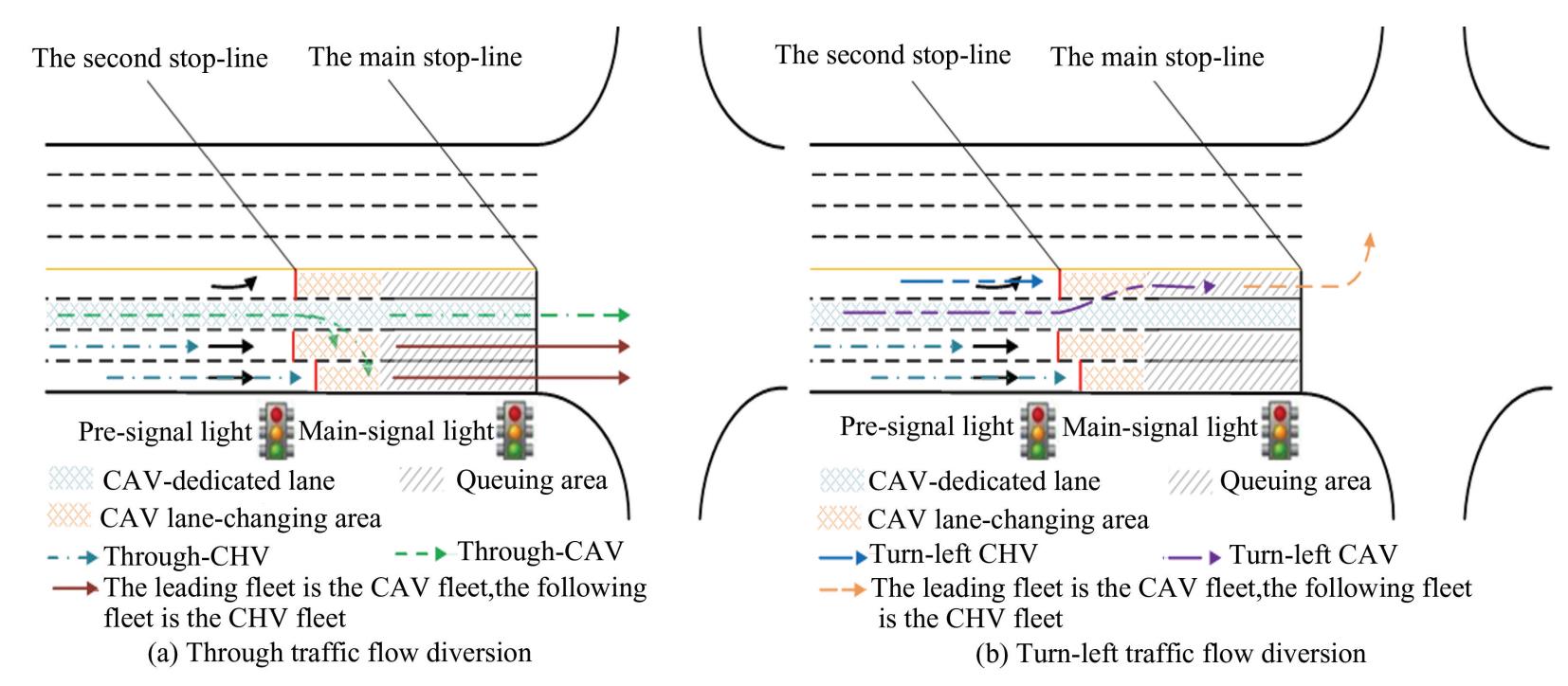
Fig.
2
Schematic diagram of traffic flow organization
1)Lane configuration.
Except for the through lane adjacent to the left-turn lane,all other approach lanes are equipped with a second stop line located downstream of the main stop line,along with pre-signal timing to separate the mixed traffic flows of CAVs and CHVs at the approach of the intersection. Additionally,the number of left turns and through lanes must be configured based on the principle of balancing the traffic volume distributed across each lane. When the number of approach lanes on road 𝑒 is three or more,the allocation method for the approach lanes at the intersection is as follows:
(20)
(21)
In these equations, represents the total number of lanes in the 𝑒th approach lane,whereas and denote the number of through and left-turn lanes at the main stop line,respectively. Additionally, refers to the number of CAV-dedicated lanes on the eth approach lane,which is set to 1. The variables and correspond to the peak-hour traffic volumes of through and left-turn CAVs on the eth approach lane,respectively. Lastly,𝛿 is the threshold used to assess lane balance in traffic volumes.
2)Location of the second stop line.
The distance between the second stop line and the main stop line should satisfy the following requirements,as shown in Fig. 3.
(22)
(23)
(24)
(25)
In these equations,Le represents the distance between the second stop line and the main stop line,and 𝐿𝑤 denotes the length of the queuing area. The length of the CAV lane-changing area is given by 𝐿𝑣,and 𝐿𝑒,𝑞 specifies the space required for queuing the CAVs in either the through(𝑞= 𝑡)or left-turn(𝑞= 𝑙)lanes of the eth approach lane. 𝑐 represents the average signal cycle over the same historical period,and 𝑑a refers to the length of the CAV. The safe distance maintained between CAVs during queuing is denoted by 𝑑ai. Additionally,𝑣𝑣 indicates the speed of vehicles while changing lanes,𝑊 is the width of a lane,and 𝜃 refers to the angle during a lane change. 𝑛 represents the total number of lanes in lane group 𝑙 and 𝑎𝑣 is the acceleration applied during lane changes.
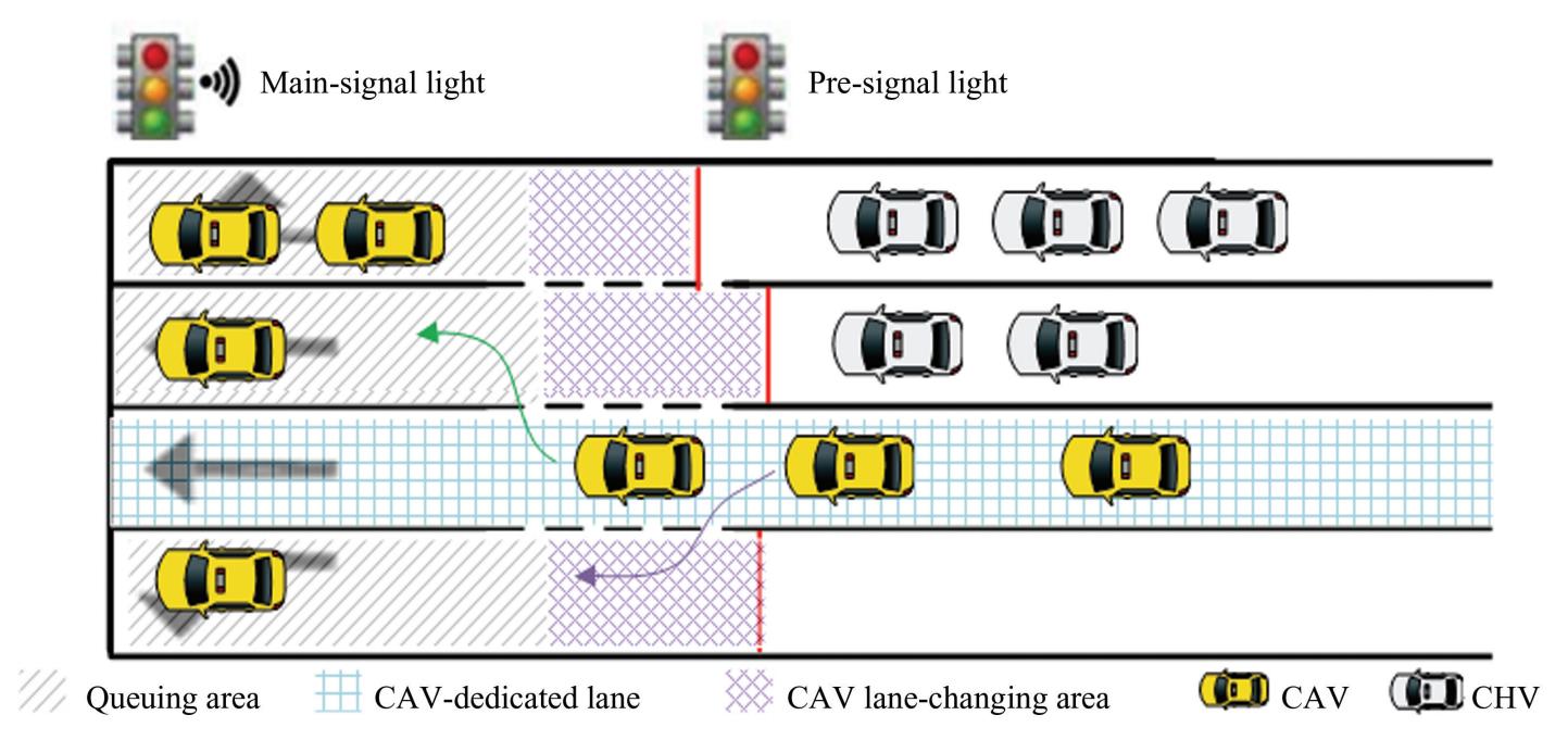
Fig.
3
Composition of 𝐿𝑒
Eq.(23)determines the length of the CAV queue area in the through(𝑞= 𝑡)/ left-turn(𝑞= 𝑙)lanes of the eth approach lane. Eq.(24)represents the calculation method for the maximum queue length of CAV. And Eq.(25)is used to calculate the length of the CAV lane-changing area. The design of fixed length 𝐿𝑒 aims to provide a stable and easy to implement foundational framework for low CAV penetration scenarios. Its core goal is to ensure that dedicated lanes can be effectively utilized under most expected traffic conditions,while avoiding the impact of overly complex designs on project feasibility.
3)Coordination relationship between the main and pre-signals.
In scenarios where the main and pre-signal cycles are identical,adjustments are necessary to minimize the loss of the main signal green time and prevent CHVs from remaining between the second stop line and the main stop line when the main signal green time ends. Specifically,the pre-signal green time should start Δ𝑡1 earlier than the main signal green time and conclude Δ𝑡2 earlier,as illustrated in Figs.4 and 5.
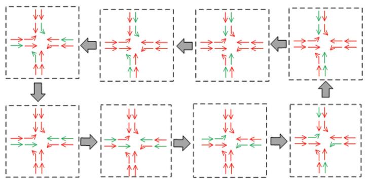
Fig.
4
Phase diagram of main-and pre-signals
(26)
(27)
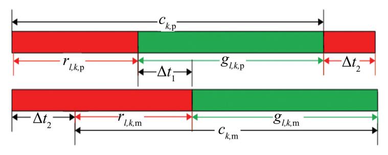
Fig.
5
Relationship between main- and pre-signals
(28)
(29)
In these equations,Δ𝑡1 represents the time at which the pre-signal green lights start before the main signal green phase,and Δ𝑡2 denotes the time at which the pre-signal green lights end earlier than the main signal green lights. vcross is the target speed of vehicles crossing an intersection stop line. indicate the start time of the main signal through the green lights in the 𝑘th cycle for lane group 𝑙,whereas specify the start time of the pre-signal through the green lights in the same cycle for lane group 𝑙. Similarly, represent the start time of the left-turn green lights in the 𝑘th cycle of the pre-signal for lane group 𝑙.
2.3 Lane-changing and Trajectory Optimization
When CAVs enter the control range,their lane changing and trajectory planning areas are shown in Fig. 6.
1)Lane changing model.
When the CAVs enter the communication range of the intersection,the signal controller optimizes their trajectories to guide them toward the main stop line. To ensure maximum lane utilization,CAVs are prioritized to change lanes toward the outermost lane,thereby mitigating the formation of long queues in the inner lanes,whereas the outer lanes remain underutilized. Simultaneously,to balance traffic flow and fully exploit available green time,the queue lengths across lanes in the same direction are regulated to ensure even distribution.
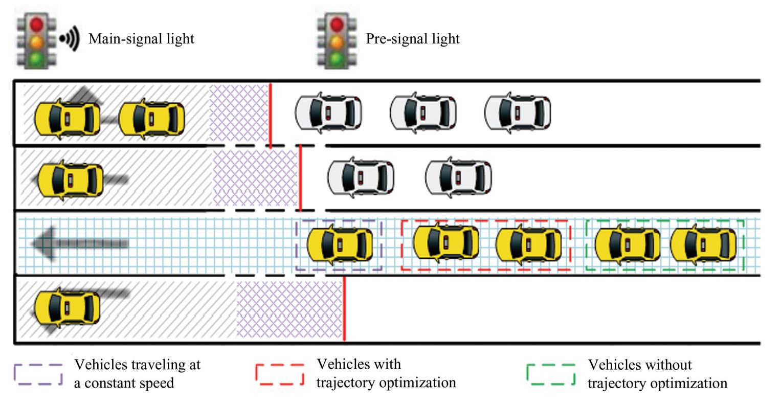
Fig.
6
Schematic diagram of CAV optimization range
The SCM-MT employs a fifth-degree polynomial for lane-changing path planning. The vehicle coordinate system was established with the centroid of the target vehicle at the initial moment of lane change as the origin,the vehicle's travel direction as the 𝑥-axis,and the direction of the lane change along the 𝑦-axis.
(30)
(31)
Here,𝑡 represents the time of lane changing,𝑡 s ≤ 𝑡 ≤ 𝑡o,and 𝑡s is the time at which the ith vehicle in lane 𝑏 of lane group 𝑙 starts changing lanes,𝑡o denotes the time when the vehicle finishes a lane change. 𝛽𝑖𝑏𝑙(𝑡)corresponds to the driving state matrix of the vehicle at time 𝑡.
2)Trajectory optimization model.
CAVs can communicate their position and speed to the signal controller and receive instructions to adjust their trajectories. This enables certain CAVs,which would normally arrive at the second stop line after the pre-signal turns green,to accelerate and enter the queue area before the pre-signal's green phase begins. The objective is to enhance traffic efficiency during the subsequent main signal green time.
(1)If a CAV can reach the queue area while maintaining its current speed during the pre-signal red phase,no trajectory optimization is required.
(32)
(2)If the CAV arrives at the queue area at a constant speed only after the pre-signal has turned green,trajectory optimization is applied. In such cases,the CAV first accelerates to the maximum speed limit,maintains that speed,and then decelerates to enter the queue area before the pre-signal green phase begins. The optimized trajectory can be expressed as follows:
(33)
Here,𝑡𝑖𝑏𝑙 is the time at which the 𝑖th CAV on lane 𝑏 of lane group 𝑙 enters the communication boundary.𝑣𝑖𝑏𝑙 denotes the speed of the 𝑖th CAV on lane 𝑏 of lane group 𝑙. If and then vehicle 𝑖 is identified as the last vehicle subject to trajectory optimization. CAVs falling outside this optimization range,even when operating at their maximum speed,will not be able to enter the queue area before the pre-signal green phase begins.Maintaining a constant speed upon entry is recommended for these vehicles.
The SCM-MT employs a uniform acceleration and deceleration strategy to optimize CAV trajectories.The process is defined as follows:
(34a)
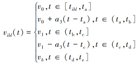
(34b)
where 𝑎₃ represents the acceleration during the uniform acceleration stage,and-𝑎₃ denotes the acceleration. The time when the vehicle enters the communication boundary is denoted as 𝑡 𝑖𝑏𝑙,𝑡 a is the initial moment of acceleration,𝑡 b represents the time at which the vehicle completes acceleration,and 𝑡 c indicates the moment the vehicle reaches a constant speed. Furthermore,𝑡 d is the time at which deceleration ends,and 𝑡 e corresponds to the moment the vehicle enters the queue area. The initial velocity of the vehicle upon entering the communication boundary is denoted as 𝑣0,𝑣1 represents the speed attained after uniform acceleration,and 𝑣b is the speed at which the vehicle enters the queue area.
2.4 Model Solution
The particle swarm optimization(PSO)algorithm is an evolutionary optimization technique inspired by the social behavior of swarms,such as birds collectively searching for food. In a 𝐷-dimensional search space,a population of 𝑛 particles is denoted as Each particle, represents a 𝐷-dimensional vector that corresponds to the position of the 𝑖th particle in the search space and serves as a feasible solution to the optimization problem. The fitness value of each particle position 𝑿𝑖 is calculated using the objective function. Each particle travels through space with a velocity which directs 𝑖ts movement. The updates for the position and velocity of each particle are governed by the following equations:
(35)
(36)
Here,the inertial weight 𝜔 is used to balance global exploration and local exploitation. The acceleration coefficients 𝑐₁ and 𝑐₂ are usually set to 2. They regulate the influence of individual optimal position 𝑷𝑖 and global optimal position 𝑮𝑖,respectively. The random numbers 𝑟₁ and 𝑟₂ follow a uniform distribution on [0,1] and introduce randomness into the search process. 𝑿(𝑖+1)and 𝑽(𝑖+1)represent the position and velocity at iteration 𝑖+1,respectively.
This study adopts a hierarchical framework to achieve joint optimization of vehicle trajectories and traffic signals. In this framework,the PSO algorithm is used as an outer optimizer specifically for optimizing traffic signal timing parameters. The execution of the particle swarm optimization algorithm follows the following steps:
Step 1:Particle swarm initialization. The algorithm was initialized with acceleration factors 𝑐₁=𝑐₂= 2,an inertia weight 𝜔= 0.8,and random numbers 𝑟₁= 𝑟₂= 1. Each particle's position 𝑿₁ represents the green times for each phase in the main signal's first cycle,and
An initial population of 30 particles was generated,with a maximum iteration count of 300.The initial velocity 𝑽𝑖 for each particle was calculated using Eqs.(6)–(19)and Eqs.(22)–(31).
(37)
In Eq.(37),𝑋𝑖 p refers to the green time of phase p in the 𝑖th particle;ℎp is the saturated headway of phase p;𝑙 p is the number of lanes in phase p;and 𝑛𝑗p is the number of vehicles forming a saturated queue in the 𝑗th lane of phase p.
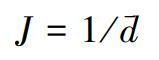
Step 2:Fitness calculation. For each particle,𝑖ts fitness 𝐽 needs to be calculated. The fitness calculation process embodies the joint optimization idea mentioned:firstly,the current particle timing scheme is taken as the given condition and input into the trajectory planning module in Section 2.3 to calculate the optimized trajectory of the CAV under this timing.Then,based on the optimized traffic flow state,the average vehicle delay 𝑑 of the entire intersection is calculated through a simulation model. Since the optimization goal is to minimize the average vehicle delay,the fitness function was defined as the inverse of this objective function to align with the PSO's maximization framework:
(38)
Here, is calculated based on Eq.(1).
Step 3:Update extremes. Based on the fitness value calculated in Step 2,the individual optimal position 𝑷𝑖 of each particle and the global optimal position 𝑮𝑖 of the swarm are updated.
Step 4:Update velocity and position. The velocity of each particle is updated according to Eq.(36). This update process takes into account the difference between the current location and 𝑷𝑖 and 𝑮𝑖.The particle position is then adjusted according to Eq.(35).
Step 5:Termination check. The algorithm then checks whether the maximum iteration count of 300has been reached. If not,the process returns to Step 2,and the iteration counter is incremented. If the termination condition is met,the algorithm concludes,and outputs the final solution.
Given a population size 𝑛,a maximum of 𝑇 iterations,and a search dimension 𝐷(the number of signal phases),updating particle velocities and positions as per Eqs.(35)and(36)incurs a cost of 𝑂(𝑛×𝐷). Therefore,the overall complexity across 𝑇 iterations is 𝑂(𝑇×𝑛×(𝐷+𝑑)),where 𝑑 represents the costs associated with the traffic delay simulation model. Under the parameters used in this study(𝑛=30,𝑇= 300,𝐷= 4),the algorithm is practically linearly scalable with runtime basically dependent on the simulation model 𝑑. The mean iteration time using these approaches is 7.59 s,which can be observed to be 9.36 s(high),5. 88 s(medium),and 7. 52 s(low). After 30 runs,SQP takes about 7.89 s,and for high,medium,and low flow rates,execution times were about 11.61,6.87,and 5.18 s,respectively. In contrast,the overall solution times of PSO are lower than those of SQP,and 𝑖ts runtimes are more stable at different flow levels.
3 Simulation Design
3.1 Basic Conditions
This study utilizes MATLAB numerical simulations to assess the effectiveness of SCM-MT.
1)The simulated intersections cover two geometric layouts:cross-shaped and T-shaped. All intersections consist of one left-turn lane,one CAV-dedicated lane,one through lane,and one shared lane for through and right-turn. The communication range of the intersection was set to 200 m with a CAV penetration rate of 25%. The second stop line was positioned 45 m upstream of the main stop line.During peak hours,the number of queued CAVs in a single lane typically ranges from 8-9.
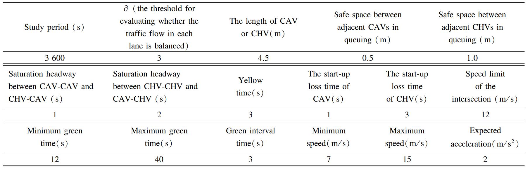
2)To facilitate the comparison of the results,the parameter values were selected based on Ref.[31],and the relevant simulation parameters are summarized in Table 1. The low(300-600 pcu/ h),medium(600-900 pcu/ h),and high(900-1200 pcu/ h)traffic volumes are listed in Table 2.
Table
1
Simulation parameter values in this study
Table
2
Traffic volumes

3.2 Scheme Design
In this study,two sets of simulation experiments that include five schemes were designed. The purpose of experiment 1 was to assess the effectiveness of SCM-MT. In this experiment,Scheme 1 implements trajectory-free optimization combined with fixed signal timing,Scheme 2 incorporates vehicle trajectory optimization while maintaining fixed signal timing,and Scheme 3 shows the SCM-MT. The key differences among the three schemes are listed in Table 3.
Table
3
Differences among the three schemes

Experiment 2 was designed to assess the performance of SCM-MT to explore its competitiveness. In this experiment,the SCM-MT was compared with the first-in-first-out(FIFO)method[36]and the phase continuous tandem intersection(PCTI)introduced by Zheng[25].
4 Result Analysis and Discussion
4.1 Simulation Result Analysis
To verify the performance of the shape,five parallel experiments were conducted under the same traffic scenario to eliminate abnormal interference.Under different traffic demands,the average results are shown in Table 4.
Table
4
Average delay of different intersections
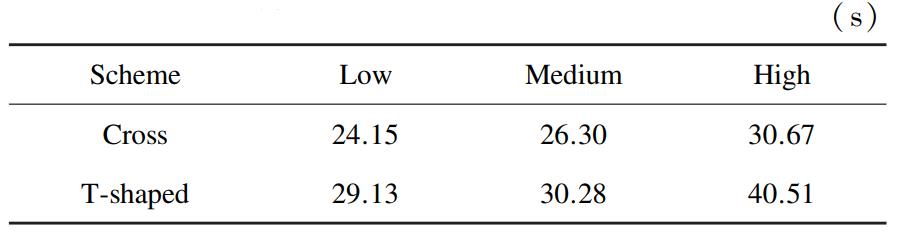
Based on the data in Table 4. The delay at the cross intersection is lower and more appropriate than the control method proposed in this paper. For that purpose,this article uses the cross intersection as a verification scenario. To test the performance of SCM-MT,we load the traffic state parameters of 12 traffic scenarios(low,medium,and high)to conduct 5experiments with the same traffic scenario. Table 5and Fig.7 show average outputs under various demands,while Fig.8 shows average fuel consumption indicators tested based on the VT-Micro model[37]in experiment 1.
Table
5
Average delay of experiment 1 under different traffic demands
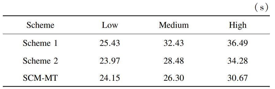
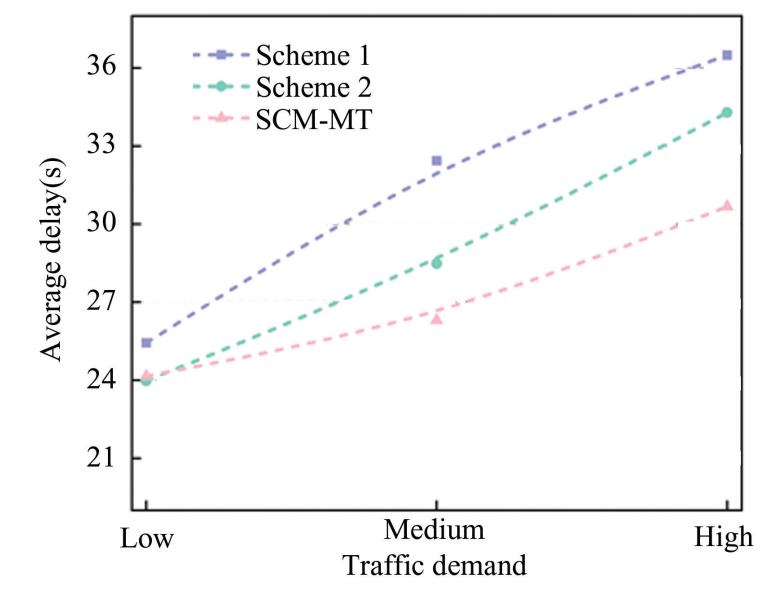
Fig.
7
Average delay of different schemes under different traffic demands
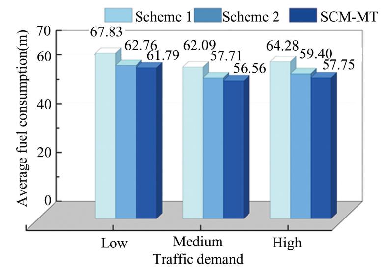
Fig.
8
Average fuel consumption of different schemes under different traffic demands
According to Table 5 and Fig. 7,the performance of SCM-MT varies with the change in traffic demand.SCM-MT outperforms other models in scenarios of high traffic. There were not many variations in the average delay of the three schemes. Most vehicles can pass a traffic signal during one cycle. This shows that under fewer pair conditions,the SCM-MT does not significantly affect average delays. When traffic demand is moderate,and both demand and the number of queued vehicles keep increasing,the signal cycle is also forced to extend. The delay gap between the different schemes has also widened,with Scheme 2and SCM-MT performing better. Especially in SCM-MT,by planning the vehicle trajectories rightly and optimizing the timing of signals,more vehicles can pass through the same green phase. This method reduces queuing delays due to long signal cycles.When demand is high,SCM-MT's benefits are even more obvious. In particular,it lowered the average delay compared with Scheme 1 and Scheme 2 by18.97% and 11. 77%,respectively. The red phase of the pre-signal was turned on earlier,which led to this gain. All CAVs can speed up within the trajectory optimization range and accelerate into the queue area beforehand. Thus,the time taken in the parking queue is reduced.
As shown in Fig. 8,the average fuel consumption of the three schemes under high demand is relatively high. The least efficient solution is Scheme 1,while SCM-MT has the least fuel consumption. Every scheme's total fuel consumption decreases with lower demand. SCM-MT keeps optimum performance in this situation. SCM-MT collaborates to optimize the trajectory and signal,which does not allow vehicles to frequently start and stop. Apart from this,the effect is enhanced by the pre-signal and dedicated lane configuration.
Fig.9 indicates that SCM-MT can optimize vehicle trajectory scheduling. CHVs might reach the intersection earlier than CAVs in reality. Through coordinating the main and pre-signal along with CAV trajectory and lane-changing optimization,CAVs can gain priority over CHVs. This unique scheduling strategy helps avoid conflicts between CAVs and CHVs,which allows for smoother traffic flow during peak times. Fig. 9 also shows a disadvantage:due to the pre-signal,some CHVs must stop at the second stop line,which degrades their performance under high traffic conditions.
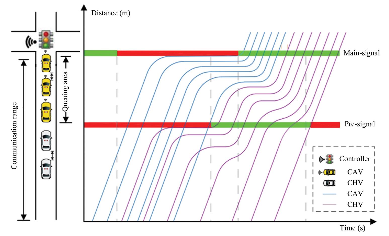
Fig.
9
Trajectories of CAVs and CHVs in a signal cycle
In order to evaluate the performance of SCM-MT,the simulation environment is still set with a road length of 200 m and a CAV penetration rate of 25%. SCM-MT is compared with FIFO and PCTI methods under low,medium,and high traffic demands. The results presented in Table 6 and Fig.10 illustrate the average delay performance and differences among the three control methods.
According to the results in Table 6 and Fig.10,under low traffic demand,the average vehicle delay in SCM-MT is slightly higher than that of the FIFO method but lower than that of the PCTI method.
Table
6
Average delay of three schemes under different traffic demands
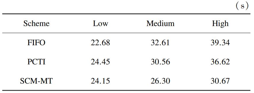
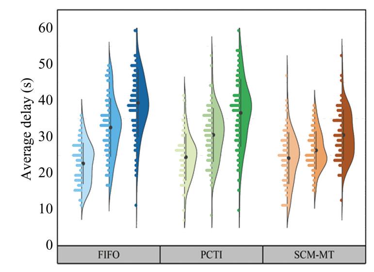
Fig.
10
Comparison of control effects among three schemes
Specifically,SCM-MT increased the delay by6.08% compared to FIFO and decreased it by 1.24% compared to PCTI. This outcome stems from the joint optimization of signal timing and vehicle trajectories in SCM-MT,which improves control performance but also introduces additional stops. The FIFO method allows vehicles to pass through intersections with minimal delay due to its simple scheduling mechanism. As a result,the advantages of SCM-MT are less evident in low-traffic scenarios. Nevertheless,SCM-MT still offers certain benefits over PCTI. PCTI mainly classifies traffic flow to reduce the cross-flow interference phenomenon between the track and the mainline. However,it does not make full use of the differences in the behavior of the types of vehicles.SCM-MT increased CAV efficiency via trajectory planning during passage,but the average delay was only slightly reduced. Although the improvement is small,it nonetheless shows the power of SCM-MT and suggests further ways for improvement.
SCM-MT shows great improvement with high traffic demand since average vehicle delay decreased by 28.27% and 19.4% when compared to FIFO and PCTI,respectively. In this scenario,the intersection faces severe congestion. The characteristics include prolonged vehicle queue time and a long signal cycle.FIFO cannot fully solve the congestion problem. It releases vehicles solely based on arrival time,without considering the vehicle type or changing traffic conditions. It results in inefficient queuing,increased delays,and dispersed distribution of delays. Traffic flow through PCTI is classified. Then,it allows straight-and left-turners to enter the queue area alternately. However,it still fails to optimize the intersection. By not taking advantage of the high maneuverability and controllability of CAVs,it loses efficacy. SCM-MT,on the other hand,takes CAVs to the queue area and forms a queue type with a shorter saturated headway[29]. With this method,more vehicles can pass in the same green phase.SCM-MT uses a release strategy that follows CAVs for CHVs,so it does not face the start-up loss time in mixed traffic.
According to the observation presented in Figs.11-12,there is considerable scatter and instability in the delay distributions of FIFO and PCTI under low,medium and high traffic. SCM-MT achieves a lower average delay and a more focused delay distribution with smaller steady-state variations. This indicates that SCM-MT performs more stably under traffic changes than other methods. FIFO performs adequately when demand is low,since queues are short and vehicle interactions are limited. However,it offers no targeted mechanism for shaping queue composition or managing dissipation. As a result,some vehicles experience unnecessary waiting time,and the overall delay distribution fluctuates considerably. PCTI did not fully exploit the dynamic characteristics of vehicles(such as the precision control capability of CAVs),which leads to limited optimization in low-flow scenario. As the queue gets longer and signal cycles increase,medium-to high-traffic demands reveal stability issues associated with FIFO and PCTI.FIFO is not capable of effectively managing the release of different vehicle types,which could cause blockages and consequently incur higher,more consistent delays with more dispersed distributions.PCTI has improved the traffic flow scheduling to an extent. However,it loses the high maneuverability and controllability of CAVs. Also,it generates large delay fluctuations under high traffic demand.
The strategy of mixed traffic increases the capacity of the intersection more than any other pre-signal strategy [20]. As a result,SCM-MT can assist in reducing the congestion caused by parking and starting too often. Additionally,it can reduce delay changes caused by the inconsistency of the dynamics of vehicles. SCM-MT introduces a secondary stop line and a pre-signal during off-peak demand. This prevents small delays from becoming large ones by planning the trajectories of CAVs while also adopting flexible signal timing. Such coordination enables smoother acceleration of vehicles and orderly queuing in the approach lanes,thereby preventing chaotic traffic behavior that usually causes variations in delays. As traffic demand increases to a medium level,the advantage of SCM-MT optimization becomes more evident. 𝐴 dramatic modification in vehicle trajectories and queue optimization for a more effective response to rapidly changing traffic conditions. The vehicle delays remain low and quite steady due to the high stability of delays. SCM-MT is also responsible for coordinating the formation of CAV compact platooning and the release of CHVs to cope with high traffic demand. This strategy shall enhance the green-time usage and improve the intersection throughput to a greater extent.
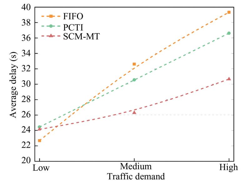
Fig.
11
Changing trend of average delay in three methods under different traffic demands
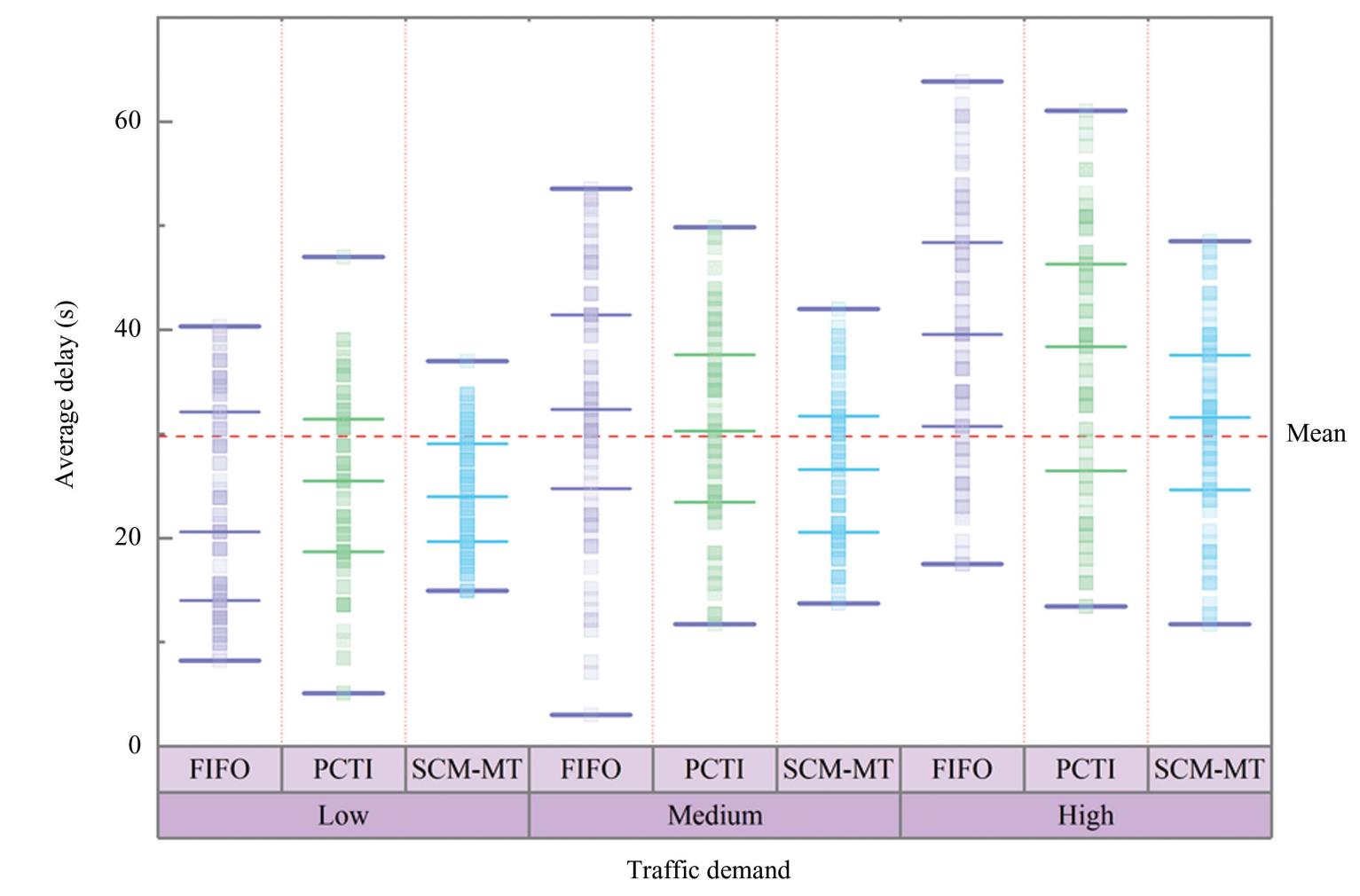
Fig.
12
Distribution of average delay for three methods under different traffic demands
4.2 Sensitivity Analysis
1)Impact of CAV penetration rate on average vehicle delay. When the road segment length is200 m,and the queue area length is 45 m,the medium traffic volume remains constant while the CAV penetration rate increases from 0.05 to 0.30,the simulation results are presented in Fig.13.
In Fig.13,a Gaussian function is used to fit the relationship between average delay and CAV penetration rate. Here,𝑦₀ denotes the baseline delay,𝑥c refers to the peak center position,𝑤 is the shape parameter controlling the peak width,and 𝐴 shows the peak amplitude. This indicates that when the CAV penetration rate is approximately 25%,the average delay reaches its minimum. According to Fig.13,the average vehicle delay fluctuates up and down as the CAV penetration rate increases. At the beginning,the delay decreased gradually,with a small rebound at the end. That is,the delay gradually decreased as the penetration rate increased. CAVs improve queue operation efficiency at low and medium levels of CAV penetration. However,when the penetration rate reaches 0.30,there is a slight increase in delay. As the penetration rate increases,we will see a reverse trend. This reversal is largely due to differences in behavior and coordination of CAVs and CHVs at medium to high penetration rates. Such differences exacerbate local traffic conflicts. The conflict partially offsets the efficiency improvement offered by CAVs.
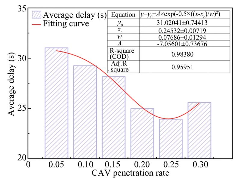
Fig.
13
The impact of different CAV penetration rates on average delay
2)Queue-area length. According to the data collected from the flow of straight lanes and left turning lanes recorded in Table 2,the lane with the largest volume of traffic will be selected for analysis to calculate the length of the queue area. The initial length of the queue area is obtained by substituting appropriate flow parameters into Eqs.(22)-(25).The length of the road should be considered as 200 m at a penetration rate of 0.25 and medium traffic. The queue size is expanded in increments of 25,35,45,55,and 60 m. The associated simulation results are shown in Fig. 14.
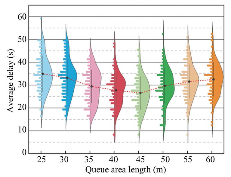
Fig.
14
The impact of queue area length on average delay
Fig.14depicts that the average delay first decreases and then increases with the queue area length. The queue area,when short,does not have sufficient length to accommodate a sufficient number of vehicles. CAVs face congestion when they navigate to the dedicated lane. As a result,some CAVs have to wait inside the lane,which is detrimental to traffic performance. When the queue length is 45 m,the average vehicle delay is at its least value. This distance is capable of accommodating vehicles while also directing them to the CAV-dedicated lane,optimizing space usage in traffic. When the queue area exceeds 60 m,it appears too long. Long queue areas can result in the wastage of road resources. At this point,further expansion of the queue area does not enhance traffic efficiency but increases the travel time of the vehicles in the queue. In the end,it lowered the utilization rate of space resources.
5 Conclusions
1)This study draws on the notable distinction between CAV maneuverability and controllability and that of CHVs. Vehicle separation,lane-changing,and queuing at the intersection are regulated through the provision of dedicated lanes,a pre-signal and a CAVs queuing area. SCM-MT aims to minimize average vehicle delay as efficiently as possible. According to the results of the simulation,the proposed method reduces the average vehicle delay by 28.27%compared to the first-come-first-served strategy and by 19.4% compared to the phase continuous tandem intersection. SCM-MT yields optimal performance under CAV penetration rates of no more than 30%.The optimal value for this scenario has been determined at a queue area length of 45 m.
2)The SCM-MT measure will add additional stops for a CHV. However,this might have adverse effects on passenger comfort. Future studies should focus on the dynamic coordination of main and pre-signals for reducing the secondary stopping of CHVs.Addressing this issue is essential for balancing efficiency and comfort in the driving experience.
Conflict of Interest
The authors declare no potential conflict of interest.
