Abstract
This study uses the classical orthogonal Laguerre polynomials as a foundation for constructing new operators. We present the Laguerre-Pǎltǎnea operator based on the modified Laguerre polynomial that facilitates the approximation of integrable functions. Furthermore, some new discrete and integral-type operators derived from the combination of the Laguerre operator, Laguerre-Pǎltǎnea operator, and Szász-Mirakyan operator are proposed. We compare the error values of the operators and emphasize which operator provides the best approximation. Ultimately, Mathematica software is utilized to generate graphs and infer the convergence of the stated operators to a function for various parameter values under consideration. Additionally, we compare each specified operator and observe that the proposed Laguerre-Pǎltǎnea operator under discussion offers a better approximation than the other potential compositions.
0 Introduction
Approximation theory is a systematic theoretical study of techniques that employ numerical approaches to solve various problems of mathematical analysis. In practice, it typically refers to the application of computer simulations and other computational methods in various scientific fields. Approximation theory, especially estimation by polynomials and piecewise polynomials, has long been closely associated with Computer-Aided Geometric Design(CAGD); where the design, calculation, and computer representation of curved shapes are the main focus of CAGD. Approximation theory is widely used in machine learning, as several machine learning algorithms rely on approximating complex functions to establish relationships between input data and output labels.
Optimization algorithms often employ approximation approaches to explore the search space and identify suitable solutions effectively. It is also an essential part of modern artificial intelligence, as it approximates complex functions by composing simpler ones using layers of interconnected neurons.
In this study, we compose various operators to define new discrete and integral type operators based on a special function, Laguerre polynomials. These polynomials are the most significant classical orthogonal polynomials. They have applications in a variety of mathematical disciplines. Additionally, these polynomials have provided numerous applications in physics, engineering, and other fields, including plasma physics, quantum mechanics, and the measurement of symmetric and central vortex states in Bose-Einstein condensates in 3-D with cylindrical symmetry[1]. Further, the computation of weights and nodes in the Gauss-Laguerre quadrature strongly depends on the evaluation of Laguerre polynomials. Here, we mention some research on generating functions, closed forms, and efficient computation of Laguerre polynomials(see Refs.[2-4]). Recently, Gupta [5] explored a discrete operator based on the modified Laguerre polynomial.
We start by recalling the well-known special function, Laguerre polynomials 𝐿𝑘(𝑥), which are solutions to the Laguerre differential equations given by:
(1)
where 𝐷𝑛 represents 𝑛-th derivative of 𝑦 with respect to 𝑥, and Eq.(1) is a second-order linear differential equation that has non-singular solutions only if 𝑘 is a non-negative integer. The closed form for 𝑘th Laguerre polynomial and the generating function, as mentioned in Ref. [2], have the following forms, respectively:
and
Now, considering the Generalized Laguerre polynomial (𝑥), for 𝛼>-1, which is defined as the following differential equation's solution:
The closed form of the 𝑘th Generalized Laguerre polynomial and the generating function, as mentioned in Ref.[4], have the following forms, respectively:
and
(2)
Remark 1 For 𝑥 ∈(-∞,0] and 𝛼>-1, we have (𝑥)> 0.
In particular,
Following the modified generating function for Generalized Laguerre polynomials, as given in Eq.(3.3) of Ref.[4], we define
(3)
Sucu et al.[4] proposed a positive linear operator for 𝑥 ∈ [0,∞) as:
(4)
where
with 𝛼>-1,𝑛 ∈ ℕ,𝑓 ∶ [0,∞)→ ℝ is a continuous function and (-𝑥)is the modified Laguerre polynomials defined by means of confluent hypergeometric series as follows:
We denote exp𝐴(𝑦)= e𝐴𝑦.
Remark 2 Taking into account Eq.(2), we obtain
1 New Integral Operator Based on Laguerre Polynomials
In many mathematical theories, estimating a function using positive linear operators is a significant concern. Summation-integral type operators have been the subject of several published works[6-15]. Here, we consider the Pǎltǎnea variant of the operator based on the well-known special function, Laguerre polynomials. Various engineering problems have unbounded domains, such as fluid dynamics, signal processing, heat transfer, and control theory. The Laguerre Pǎltǎnea operators are very useful to address these problems. These operators act as a bridge between practical modeling requirements and theoretical approximation concepts. To solve differential equations, optimize system responses, and enhance computational algorithms, these operators have proven to be an interesting mathematical foundation. Thus, they highlight the increasing importance of this synthesis of pure mathematics and applied mathematics in modern engineering science. Some examples of this connection can be found in Refs.[16-19]. Consider the Laguerre-Pǎltǎnea operators for 𝜌> 0, α>-1 and for 𝑥 ∈ [0,∞) given by
(5)
where
with the inner product provided by〈𝑓,𝗀〉= 𝑓(𝑠)𝗀(𝑠)d𝑠,and 𝑓:[0,∞)→ ℝ is an integrable function for which the above integral and series converge. We can also consider the integral representation of Eq.(5)given by:
where
and 𝛿(𝑦) is the Dirac delta function, the so-called inverse Laplace transform of 1.
Proposition 1 The function that generates the moments for the operator is given by
Proof Consider
Utilizing Eq.(3), we have
On simplifying further,we get the required result.
Lemma 1 Using Proposition 1,we conclude that for certain constants 𝑏𝑖 and 𝑒𝑖(𝑡)= 𝑡𝑖,𝑖= 0,1,2,…,𝑏𝑖 ≠ 0,we have
Further,for some constants 𝑐𝑖,𝑖= 0,1,2,…,𝑐𝑖 ≠ 0,we have
Denote
Theorem 1 For 𝑓 ∈ 𝐶𝐵𝐷(ℝ+)(the class of all bounded functions on the non-negative real axis which are continuous),𝑟 ≥ 1,𝑠 ∈ ℝ and 𝑥 ∈ [0,∞),the subsequent limits hold true:
1)
2)
3)
Proof Using Proposition 1,with i denoting the imaginary part consider
Next
where 𝐼Id denotes the identity operator. Finally
where is a positive linear operator based on Laguerre polynomials given by Eq.(4) with moment-generating function as indicated in Remark 2.
Following Theorem 1 of Ref.[20]and references therein, we get the desired outcomes.
Consider the well-known Szász-Mirakjan operator on the class 𝐶[0,∞) defined as
Here, we introduce a new Pǎltǎnea operator which arises as the combination of Szász-Mirakyan operator 𝑆𝑛 with Laguerre Pǎltǎnea on the space 𝐶[0,∞):
where “∘” represents the composition of two operation,and
Lemma 2 For some real parameter 𝐴,the following equation holds:
For certain non-zero constants 𝑎𝑖,𝑖= 0,1,2,…,we have
2 Some New Discrete Operators Based on Laguerre Polynomials
A new discrete operator can be evolved using the Laguerre-Pǎltǎnea and Szász-Mirakyan operators. The composition of Laguerre-Pǎltǎnea operators with the Szász-Mirakyan operators 𝑆𝑛 on some subspace of 𝐶[0,∞) for which exists, can be defined as follows:
(6)
Theorem 2 A concise form for is provided by
where
and for 𝑘 ≥ 1,
Proof Eq.(6)can be rewritten as:
All the terms involved here,under sum and integration,are non-negative. Using Tonelli's theorem,we can express the above form as follows:
where
Thus
Finally,the concise form for Eq.(6)is given by
where
and for 𝑘 ≥ 1,
Theorem 3 The following holds:
Proof Taking into account Proposition 1,we obtain
Simplifying further,we get the desired results.
Corollary 1 For certain non-zero constants 𝑏𝑖,𝑖= 0,1,2,…,we have
The proof follows from the computations based on Theorem 3.
Theorem 4 For 𝑓 ∈ 𝐶BD(ℝ+),𝑟 ≥ 1,𝑠 ∈ ℝ and 𝑥 ∈ [0,∞),the following limits hold true:
1)
2)
Proof Using Theorem 3,we have
Next
Following Theorem 1 of Ref.[20] and references therein,we get the desired results.
Theorem 5 [ 21 ] Let 𝑓 ∈ 𝐶[0,∞),and [𝑎,𝑏] is a closed and bounded subinterval of [0,∞). Then,for 𝑥 ∈ [𝑎,𝑏] and any positive linear operator 𝐿𝑛 preserving constant functions,we have
Proof Consider
Choosing 𝛿 ∶= 𝛿𝑛(𝑥)= on [𝑎,𝑏],we get the required result.
Next,we produce two new discrete operators:,which is created by composing the Laguerre operator proposed by Sucu et al. [ 4 ] and defined in Eq.(4)with the Szász-Mirakyan 𝑆𝑛;and ,which is created by composing Szász-Mirakyan operator 𝑆𝑛 with ,for the functions on the space 𝐶[0,∞)for which and exist respectively.
1)The first composition has the following succinct form:
where
2)The next composition has the succinct form given by:
where
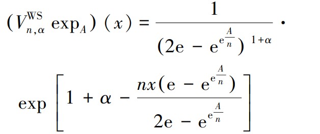
Lemma 3 The moment-generating function for and are given by:
1)
2)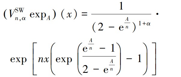
Proof Consider
Using Remark 2,we achieve the required result. Similary,we obtain the second outcome.
Lemma 4 For certain constants 𝑐𝑖,𝑖= 0,1,2,…,𝑐𝑖 ≠ 0,we have
and
Proof follows from the calculation and Lemma 3. We skip the details.
Theorem 6 For 𝑓 ∈ 𝐾 ⊂ 𝐶BD(ℝ+),where 𝐾 includes functions for which and both exist. If 𝑓″ exists at some point 𝑥 ∈ ℝ+,then we have
Applying Lemma 4 with Taylor's expansion of 𝑓 generates the proof. We omit the details.
Theorem 7 For 𝑓 ∈ 𝐶BD(ℝ+) and 𝑥 ∈ ℝ+,we have
Proof Taking into consideration Lemma 3,we get
Following Theorem 1 of Ref. [20], we obtain the result.
Remark 3 The use of Lemma 3, Lemma 4 and Theorem 6 yields the following conclusion: the two operators, and , are not equal on some subspace of 𝐶[0,∞) where both exist; rather, they are compositions of operators, namely, modified Laguerre and Szász operator 𝑆𝑛, but in a different order. They have the same Asymptotic formula.
3 Numerical Comparison of Errors
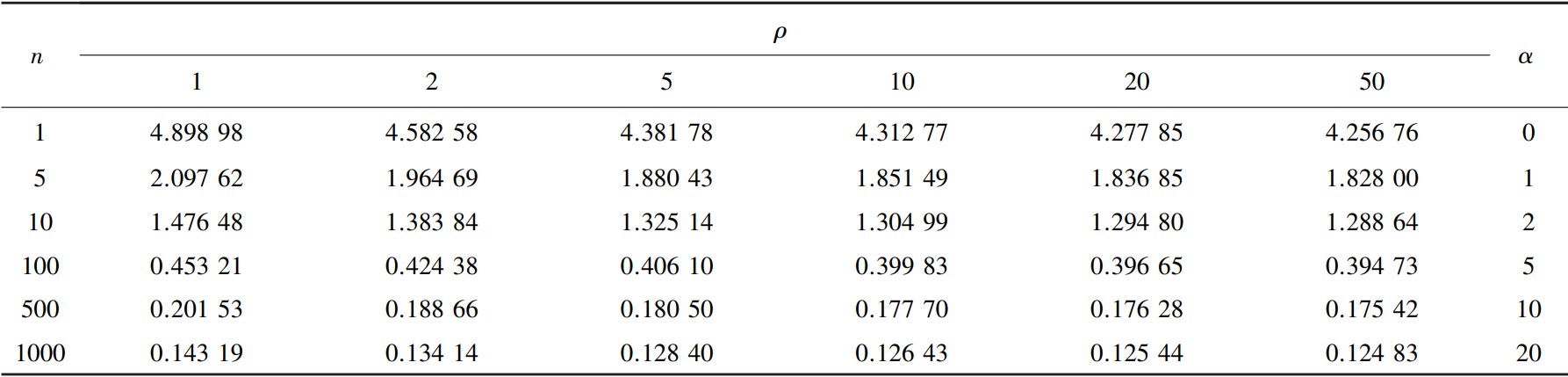
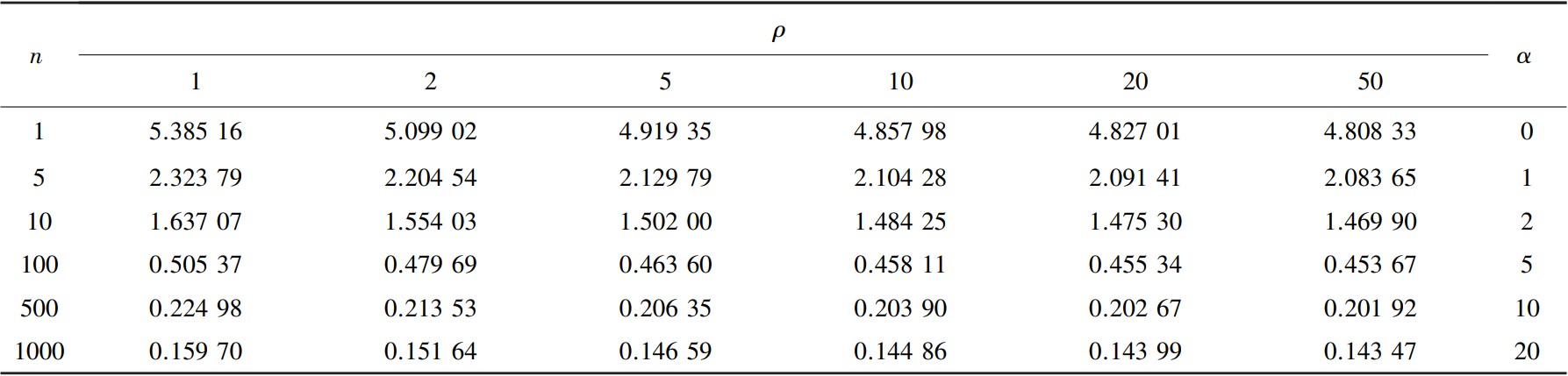
We compare the convergence of the operators, namely Laguerre Pǎltǎnea , composition of Szász with Laguerre , and composition of Laguerre with Szász , and interpret the error quantitatively in view of Theorem 5. We denote (𝑥) to be the square root of the second central moment for the positive linear operators under consideration in this paper.
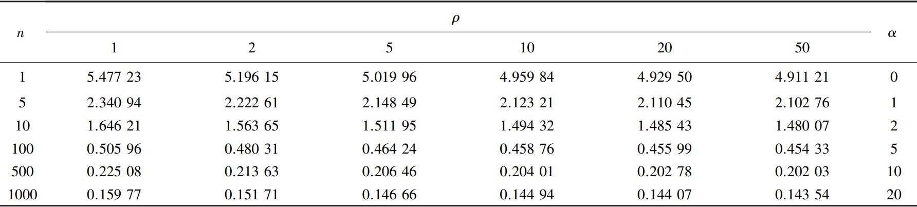
From Tables 1-3, it can be concluded that for the three operators , and defined on some subset of 𝐶[0,∞), the error term for 𝑥 ∈ [0,5] ⊂ [0,∞) reduces when either 𝑛 increases, 𝜌 increases or 𝛼 increases. However, by comparing the error values among the three above-mentioned operators, we may infer that in some closed and bounded subinterval of [0,∞), the convergence is better(or the error is smaller) for the Laguerre Pǎltǎnea operator , followed by the composition of Szász with Laguerre and, finally, the composition of Laguerre with Szász . Similar comparisons can also be made for the other operators on contracted or extended subintervals of [0,∞) and for various other values of 𝑛, 𝜌 and 𝛼.
Remark 4 Using Corollary 1, Lemma 2, and the observation made in Section 3, a conclusion can be drawn that we obtain two different operators and with different convergences properties, even though they are the composition of Laguerre-Pǎltǎnea with Szász in different orders.
Table
1
An upper bound (𝑥) on the error term for on the subinterval [0,5]
Table
2
An upper bound (𝑥) on the error term for on the subinterval [0,5]
Table
3
An upper bound (𝑥) on the error term for on the subinterval [0,5]
4 Graphical Comparison Between Operators
From Figs.1-7, we analyze the convergence of the operators for a continuous function f(𝑥)=𝑥·e-𝑥.
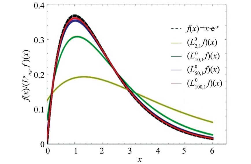
Fig.
1
Convergence of (𝑓)(𝑥)for 𝑓(𝑥)= 𝑥·e-𝑥
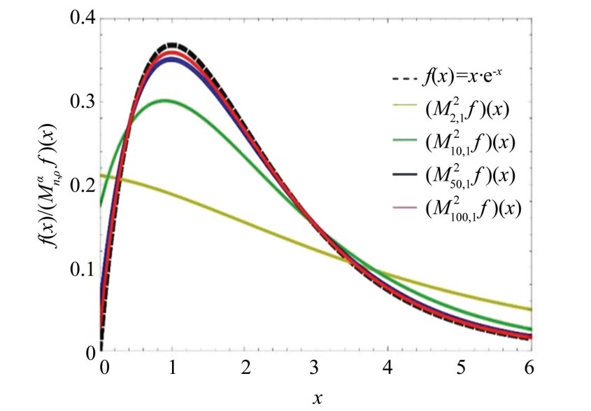
Fig.
2
Convergence of ()(𝑥)for 𝑓(𝑥)= 𝑥·e-𝑥
Figs.1-5 represent the convergence of operators , , , , and , respectively, for a continuous and infinitely differentiable function 𝑓(𝑥)=𝑥·e-𝑥. We can conclude that for some specific values of 𝜌> 0 and 𝛼>-1, increasing the value of 𝑛 enhances the convergence of the related operator to the considered function. Figs.6 and 7 compare the convergence of all the operators with 𝑛=10 and 50. We may infer that the Laguerre-Pǎltǎnea operator provides the best convergence. is followed by , , and finally . Similar comparisons can be made for various other functions and different values of parameters 𝜌 and 𝛼.
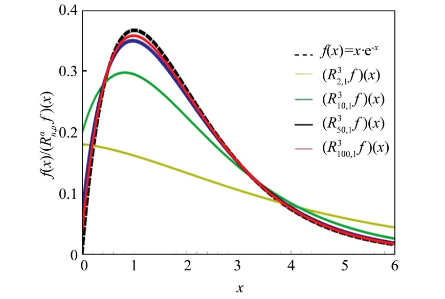
Fig.
3
Convergence of (𝑅3 𝑛,1 𝑓)(𝑥)for 𝑓(𝑥)= 𝑥·e-𝑥
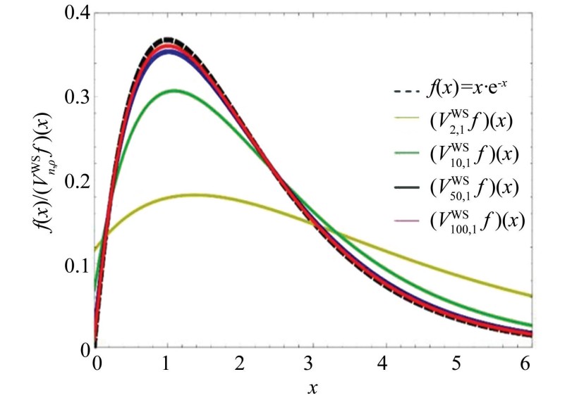
Fig.
4
Convergence of ()(𝑥)for 𝑓(𝑥)= 𝑥·e-𝑥
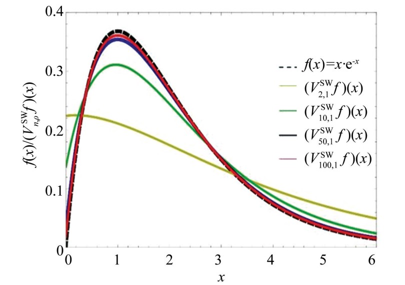
Fig.
5
Convergence of ()(𝑥)for 𝑓(𝑥)= 𝑥·e-𝑥
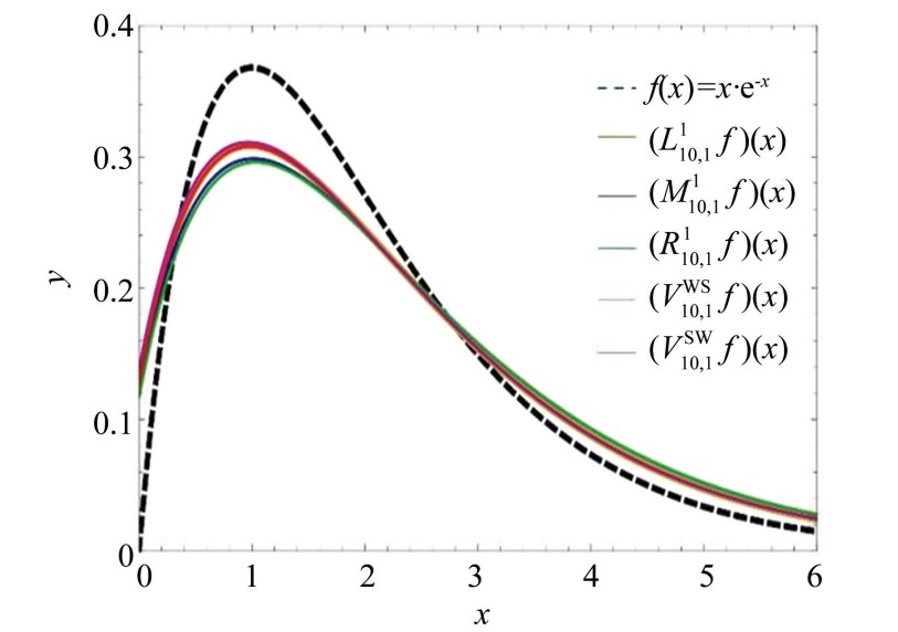
Fig.
6
Convergence for 𝑓(𝑥)= 𝑥·e-𝑥 for 𝑛= 10
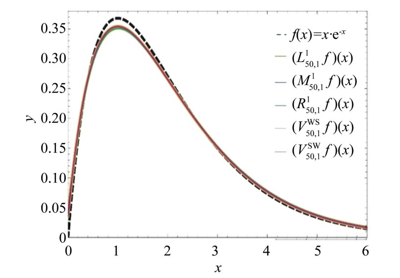
Fig.
7
Convergence for 𝑓(𝑥)= 𝑥·e-𝑥 for 𝑛= 50
5 Conclusions
In this study, we investigate approximation properties of Laguerre-type operators, with a particular focus on the Laguerre-Pǎltǎnea operator defined by modified Laguerre polynomials. We further constructed new families of integral and discrete operators by combining the Laguerre, Laguerre-Pǎltǎnea, and Szász-Mirakyan operators. Analytical results are complemented by numerical and graphical analyses using Mathematica software to examine convergence properties and approximation behavior.
From Tables 1-3, it can be concluded that for the operators , and , the error decreases as the parameters 𝑛,𝜌 or 𝛼 increase. Among these, the Laguerre-Pǎltǎnea operator consistently provides better convergence, followed by the Szász-Laguerre composition and, lastly, the Laguerre-Szász composition in some compact subinterval of [0,∞).
The graphical analysis reinforces these observations. For the test function 𝑓(𝑥)=𝑥·e-𝑥, all operators provide good convergence as 𝑛 increases, but the Laguerre-Pǎltǎnea operator demonstrates the strongest approximation. The comparative graphs indicate the following hierarchy of performance: exhibites the best convergence, followed by , , , and finally . Overall, our findings highlight that the Laguerre-Pǎltǎnea operator is the most effective among the considered operators in terms of convergence and error reduction. These results not only validate the effectiveness of this operator but also suggest new directions for further study of Laguerre-based approximation processes under different parameter regimes and for broader classes of functions.
