Abstract
In rocket booster recovery missions, robust visual perception is critical for real-time localization and landing control, but complex environments, including noise, illumination variations, and occlusion, severely degrade the accuracy, repeatability, and localization precision of traditional corner detectors, often resulting in false detections, missed keypoints, and reduced real-time reliability.To address these challenges, an Adaptive Robust Harris (ARH) corner detection algorithm is proposed in this study. The method integrates four innovations: 1) Scharr operator-based gradient computation for enhanced edge response; 2) An adaptive thresholding via statistical analysis of Harris responses to improve noise robustness; 3) A hybrid approach combining dilation-accelerated Non-Maximum Suppression (NMS) and sub-pixel refinement using OpenCV's goodFeaturesToTrack, reducing redundancy and achieving precise localization (average displacement: 0.0458 pixels); 4) Vectorized computation replacing explicit loops, optimizing runtime by 40%. Experimental validation demonstrates ARH's superior performance: high repeatability (≈0.85) under Gaussian noise, 20% feature reduction in motion blur (vs. 21% for Harris and 82% for SIFT), and stable keypoints under rotation. Computational complexity analysis reveals that adaptive thresholding is optimized from 𝑂(𝑁) to 𝑂(1), while NMS efficiency improves by 50%. These advancements position ARH as a high-precision, real-time solution for vision-critical tasks in aerospace applications, such as tracking rocket boosters and providing landing assistance.
0 Introduction
In missions involving rocket booster recovery[1], reliable and precise visual perception plays an indispensable role in real-time positioning, trajectory calculation, and final control of landing processes. Among visual features, corner points[2] are particularly important due to their spatial stability and repeatability, which are essential for downstream tasks such as feature matching[3], visual tracking[4], and 3D reconstruction[5]. During the high-speed descent of a rocket booster, the vision system must identify and track multiple high-feature-density regions to ensure accurate navigation[6]. However, environmental factors such as lighting variation, Gaussian noise, occlusion, lens contamination, and motion blur can severely affect the reliability and repeatability of corner detection algorithms[7].
The traditional Harris corner detection algorithm[8] is well-regarded for its simplicity, computational efficiency, and strong edge response under standard imaging conditions. However, it has notable drawbacks when applied to dynamic or degraded imagery. Specifically, Harris is sensitive to manually defined parameters, and its fixed-threshold mechanism often results in clustered corners in textured regions while failing to detect key points in low-contrast or noisy areas. These limitations reduce the algorithm's robustness and hinder its ability to support precise localization tasks in complex aerospace environments, especially when fast decision-making and minimal delay are required.
To address the inherent limitations of traditional Harris corner detection, researchers have developed numerous enhanced approaches that demonstrate superior adaptability and performance[9]. These improvements primarily focus on six technical directions: 1) Feature enhancement and scale invariance, exemplified by SIFT's Gaussian scale-space construction[10-11], though its computational intensity limits real-time applications[12]; 2) Computational efficiency optimization demonstrated by ORB's combination of FAST detection with BRIEF descriptors[13], achieving balanced speed and accuracy for resource-constrained environments[14]; 3) Hybrid methodologies[15-18], including PCA-optimized ORB for improved feature matching[19], Canny-based Harris refinements for edge-aware localization[20], and Harris-FAST integration for enhanced robustness[17,21]; 4) Adaptive techniques employing dynamic thresholding[22] and progressive Non-Maximum Suppression(NMS)[23] to handle noisy conditions; 5) Environment-specific solutions for challenging scenarios like underwater imaging[16,24-25]; and 6) Emerging deep learning approaches that learn complex features[26], albeit with computational constraints.
Despite these advancements, the fundamental trade-offs between real-time performance, detection accuracy, and environmental adaptability remain a critical barrier for vision systems in rocket booster recovery scenarios, where rapidly evolving visual conditions demand simultaneous robustness, precision, and speed. To bridge this gap, this study introduces an Adaptive Robust Harris(ARH) corner detection algorithm to address the aforementioned limitations of conventional Harris through the following four innovations:1) Enhanced gradient estimation using the Scharr operator to achieve high edge response sensitivity in complex texture regions[18];2) A statistical adaptive thresholding strategy that adjusts dynamically to the distribution of corner responses, eliminating the need for manual threshold selection[22,27];3) Efficient non-maximum suppression via morphological dilation, significantly reducing redundant feature points and improving keypoint separation[28];4) Sub-pixel refinement using OpenCV's goodFeaturesToTrack, ensuring high localization precision and geometric accuracy.
This research aims to develop an advanced corner detection solution that simultaneously addresses three critical requirements for aerospace applications: enhancing detection accuracy and robustness under challenging operational conditions typical of rocket booster recovery scenarios, optimizing computational performance to satisfy stringent real-time processing constraints onboard the spacecraft, and rigorously validating the proposed ARH algorithm through comprehensive testing encompassing both synthetic benchmarks and actual flight imagery to evaluate its performance across diverse interference conditions including sensor noise, motion blur, and partial occlusion. The integrated approach seeks to bridge the gap between theoretical corner detection performance and practical implementation requirements in space systems.
1 An Improved Corner Detection Algorithm Based on Harris(ARH)
The rocket booster recovery process, as the core technology of reusable aerospace systems, directly determines the success or failure of the mission through spatiotemporal coordination of its operational sequence. As shown in Fig.1, the process begins with navigation control and speed adjustment during the booster's final flight segment. When the rocket enters the 300 m range of the launch capture tower(rocket approach phase), the attitude adjustment subsystem is required to adjust the heading angle accuracy. At this point, the dual-redundancy mechanism formed by the buffer device and capture arm enters the preparatory state. The visual perception system plays a critical role in this phase: by detecting high-feature point areas in real time, the system achieves millimeter-level positioning through feature point spatial coordinate calculations. The accuracy of this detection directly affects the timing of the capture arm deployment and the engagement of the locking mechanism. However, traditional feature detection methods are prone to feature drift under dynamic lighting conditions and partial occlusion, leading to cumulative errors in the navigation control loop. To address this, the ARH algorithm proposed in this paper introduces a multi-scale gradient response fusion mechanism and dynamic threshold compensation strategy, significantly enhancing visual positioning robustness under complex conditions, while maintaining real-time performance. The following sections describe the specific process of the algorithm.
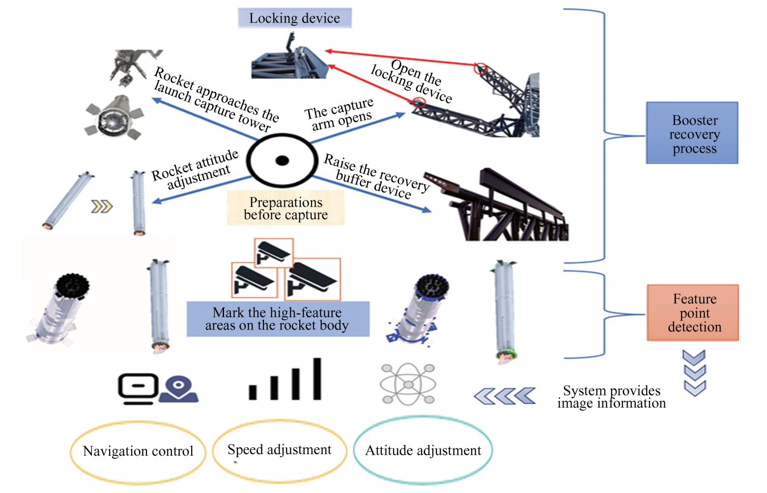
Fig.
1
Multimodal control system architecture for reusable rocket boosters: integrated navigation adjustment, feature detection, and robotic arm coordination
1.1 The Basic Principle of Harris Corner Detection
Harris corner detection is a classic algorithm based on gradient variations in grayscale images. Its fundamental concept involves evaluating local intensity changes in the image to identify corners. Typically, corners are points with significant intensity variation or intersections of edges within the image.
Assuming the grayscale value of an image is represented as 𝐼(𝑥,𝑦), and a small displacement(𝑢,𝑣) is applied to the image, the change in grayscale value can be represented by the autocorrelation function as follows:
(1)
here, 𝑤(𝑥,𝑦)is a weighted window function, typically a Gaussian function, used to reduce the impact of noise. By applying a Taylor expansion to the expression and neglecting higher-order terms, the intensity variation 𝐸(𝑢,𝑣) can be represented as:
(2)
here, 𝑴 is the autocorrelation matrix, defined as follows:
(3)
The matrix 𝑴 contains gradient information of the image in a local region, with its two eigenvalues, λ1 and λ2, describing the intensity variations. Specifically:
When both λ1 and λ2 are large, indicating significant changes in both directions, suggesting that the region is a corner.
When one eigenvalue is large, and the other is small(i.e., λ1 ≫ λ2 or λ1 ≪ λ2), it implies the presence of a distinct edge in the region.
When both eigenvalues are small, it indicates minimal intensity variation, suggesting that the region is flat.
1.2 Definition of the Corner Response Function
To avoid directly computing the eigenvalues, Harris proposed a simplified response function(𝑅), which approximates the relationship between the eigenvalues using the determinant and trace of the matrix:
(4)
where 𝑘 is an empirical constant, typically ranging from 0.04 to 0.06. det(𝑴) represents the determinant of matrix 𝑴, expressed as λ1 λ2:
(5)
A larger determinant value indicates more significant gradient changes in the region, suggesting it is likely a corner.
𝑇trace(𝑴) represents the trace of matrix 𝑴, which is the sum of the two eigenvalues, λ1+ λ2:
(6)
A larger trace value indicates significant intensity variation in the region, but it does not confirm the presence of a corner; it may indicate an edge.
Matrix 𝑴 can be represented using the smoothed results:
(7)
and:
(8a)
(8b)
(8c)
where 𝐼𝑥 and 𝐼𝑦 represent the image gradients in the 𝑥 and 𝑦 directions, respectively. 𝐺𝜎 is a Gaussian window with a standard deviation of 𝜎. The symbol* denotes the convolution operation.
1.3 Advantages of the Corner Response Function
1) Stability: Due to the use of Gaussian weighting and matrix representation, the Harris algorithm exhibits good robustness against noise.
2) High efficiency: Compared to directly computing the eigenvalues of the matrix, the use of determinant and trace approximations reduces computational complexity.
3) Robustness: Harris corner detection demonstrates strong robustness to image rotation and to certain levels of noise variation.
Using the aforementioned corner response function, the Harris algorithm can efficiently and stably detect corners in images, providing a foundation for subsequent tasks such as image matching, tracking, and recognition.
1.4 Principles of the Improved Algorithm
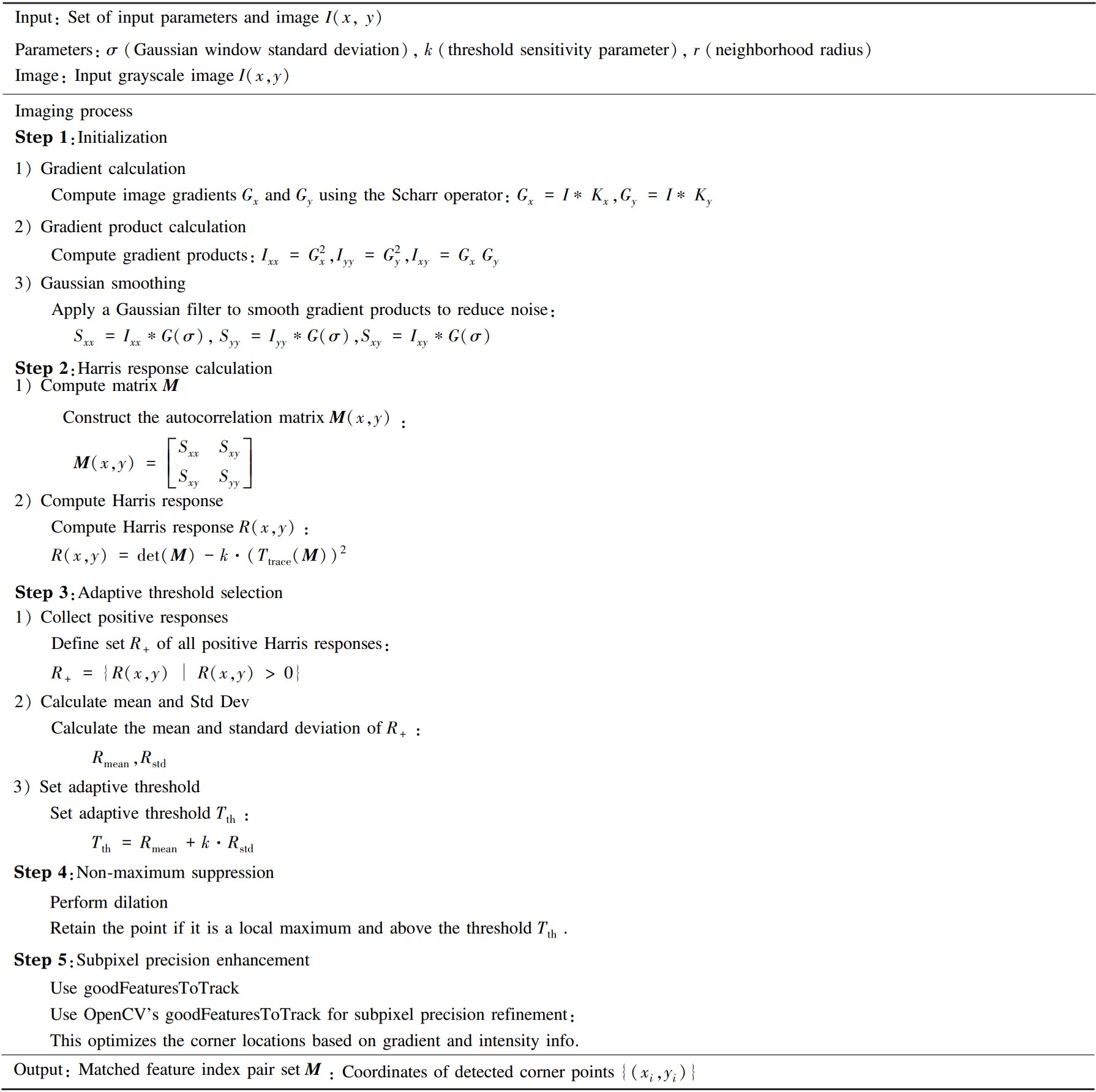
The imaging procedure of the improved Harris algorithm is as follows.
Explanation of steps:
1) Step 1(Initialization):Construct gradient maps using Scharr operators for a more accurate edge response.
2) Step 2(Harris response calculation):Use the autocorrelation matrix to evaluate the local change of intensity, which indicates the corner's presence.
3)Step 3(Adaptive threshold selection):Compute an adaptive threshold based on the statistical properties of the Harris response to adapt to different noise and contrast levels.
4) Step 4(Non-maximum suppression):Dilation is used to retain only the local maxima, ensuring isolated corners are detected while discarding neighboring detections.
5) Step 5(Subpixel precision enhancement):The goodFeaturesToTrack function helps refine detected corners, ensuring subpixel-level accuracy for subsequent applications.
1.5 Adaptive Thresholding Method
To achieve adaptive thresholding, we performed a statistical analysis of the positive 𝑅 values:
1) Collect positive 𝑅 values.
Define the set 𝑆:
(9)
2) Computation of statistical measures.
Calculate the mean 𝜇𝑅 and standard deviation 𝜎𝑅 of set 𝑆:
(10)
(11)
where 𝑁 is the number of elements in set 𝑆.
3) Define the adaptive threshold 𝑇th.
Set the threshold 𝑇th as:
(12)
where 𝑘𝑡 is a parameter that controls the sensitivity of the threshold. A larger 𝑘𝑡 results in a higher threshold, leading to fewer detected corners.
4) Principle of the method.
Determine 𝑇th based on 𝜇𝑅 and 𝜎𝑅:
a) Adaptive to image content: 𝑇th is adjusted according to the distribution of corner responses within the image.
b) Enhanced robustness: Reduces the impact of outliers and adapts to varying contrast and noise levels.
c) Improved detection performance: Achieves a balance between detecting true corners and suppressing false detections.
1.6 Non-Maximum Suppression(NMS)
During corner detection, multiple adjacent corners may be generated, which can be considered as false corners or corner clusters. To eliminate these false corners, the algorithm uses Non-Maximum Suppression(NMS) to retain only the strongest corner in the local region. Mathematically, NMS can be represented as:
(13)
where 𝑅(𝑖,𝑗) is the Harris response value at the point(𝑖,𝑗); 𝑟 is the suppression radius, defining the range of the local neighborhood.
Only when the current pixel 𝑅(𝑖,𝑗) is the maximum value within its neighborhood is it retained; otherwise, it is set to zero.
Fig.2 illustrates how NMS improves corner detection. Fig.2(a) shows the initial corner response, with multiple bright regions indicating potential corners. These regions may contain several detections of the same feature, leading to redundancy and increased errors. Fig.2(b) displays the corner detection result after NMS, which retains only the strongest response in each region, eliminating redundant detections and improving precision. By reducing noise and extraneous points, NMS produces a more focused set of corners, which is crucial for subsequent image processing tasks such as feature matching and tracking.
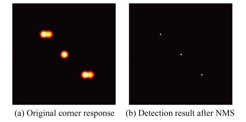
Fig.
2
Comparison of corner detection before and after NMS
Traditional NMS is typically implemented by searching for the maximum value within the local neighborhood of each pixel, often involving nested double for loops with a computational complexity of 𝑂(𝑁×𝑟2), where 𝑟 is the neighborhood radius, and 𝑁 is the number of pixels.
To optimize this process, the algorithm uses the dilation operation in OpenCV to perform NMS. The dilation operation finds the maximum value within each local neighborhood through a sliding window, and its highly optimized low-level implementation effectively reduces computational load:
Mathematical description of the dilation operation is as follows:
(14)
where 𝑁(𝑖,𝑗) represents the neighborhood centered at(𝑖,𝑗). The dilation operation is implemented in parallel, which significantly reduces the runtime.
By finding and retaining the local maximum at the same position in the original image, the dilation operation greatly improves the speed of NMS and ensures that only the strongest local corner responses are preserved.
1.7 Sub-pixel Precision Corner Position Correction
To further enhance the precision of corner positions, the algorithm refines corner locations by calculating the arithmetic mean of the corner points within their neighborhoods. This step allows the corner positions to achieve sub-pixel accuracy.
Given the neighborhood 𝑁(𝑖,𝑗) of a corner, the mean position of all corners within this neighborhood can be calculated using the following formula:
(15a)
(15b)
where 𝑥avg and 𝑦avg are the refined corner positions. 𝑁(𝑖,𝑗) represents all corner points within the neighborhood centered at(𝑖,𝑗) with a radius 𝑟, 𝑁(𝑖,𝑗) is the number of corner points within the neighborhood.
In the original algorithm, this process was implemented manually. In the improved version, the OpenCV function goodFeaturesToTrack is used to achieve sub-pixel refinement of corner positions.
goodFeaturesToTrack finds corners using the minimum eigenvalue method and allows configuration of quality level and minimum distance parameters. This approach provides a more efficient way to extract and accurately locate corners.
Mathematically, the function calculates the positions of interest points based on the gradient information of the image, utilizing a highly optimized implementation.
By using goodFeaturesToTrack, not only is the accuracy of corner positions improved, but the additional computational complexity associated with manually iterating to calculate the mean is significantly reduced.
1.8 Gradient Calculation Improvement: Using the Scharr Operator
Gradient calculation(Scharr vs. Sobel Operators): Both the Sobel and Scharr operators are used to calculate image gradients to highlight edges and corners. The Scharr operator is an improved version of the Sobel operator, employing different convolution kernel parameters to enhance edge detection in more complex images. Specifically, when calculating gradients in the 𝑥 and 𝑦 directions, the Scharr operator reduces the attenuation of high-frequency responses seen with the Sobel operator, resulting in more accurate gradient computation.
Mathematically, the Sobel operator uses a 3×3 convolution kernel for gradient estimation:
(16a)
(16b)
The Scharr operator uses optimized kernel parameters:
(17a)
(17b)
Compared to the Sobel operator, the Scharr operator reduces directional bias in edge detection by optimizing weighting, providing better edge responses and more accurate corner localization. Therefore, in this algorithm, the Scharr operator is used to accelerate gradient computation and improve corner-detection accuracy.
1.9 Vectorized Computation Instead of Explicit Loops
When calculating the response value 𝑅, the improved algorithm uses vectorized operations instead of explicit Python loops. The advantage of this approach is that vectorized computations can more efficiently leverage modern CPUs or GPUs for parallel processing.
In adaptive threshold calculation: The original calculation involved looping through 𝑅 values to compute the mean and standard deviation, which is highly time-consuming in Python. Vectorized operations utilize NumPy functions to calculate the mean 𝜇𝑅 and standard deviation 𝜎𝑅. These functions are internally optimized using low-level C language and multithreading acceleration.
The vectorized formula is:
(18)
This improvement effectively reduces the time complexity from 𝑂(𝑁) to a near 𝑂(1) complexity through low-level implementation(using multithreaded parallel processing).
1.10 Advantages of the Improved Algorithm
1) Enhanced detection accuracy: The algorithm employs the Scharr operator for gradient computation, combined with NMS and sub-pixel refinement, resulting in improved corner detection and precise feature localization.
2) Increased resistance to interference: Adaptive thresholding enables dynamic adjustments based on image content, enhancing robustness to noise and lighting variations. This leads to greater stability and reliability in detection.
3) Improved computational efficiency: The enhanced algorithm achieves approximately 40% greater efficiency than the traditional Harris algorithm by using the Scharr operator and vectorized operations, eliminating explicit loops. NMS efficiency is further improved through dilation operations.
4) Adaptive and automated parameter adjustment: The integration of adaptive thresholding and NMS eliminates the need for manual parameter tuning, ensuring consistent performance across diverse environments, especially in real-time applications.
5) High repeatability and stability: The algorithm demonstrates high repeatability under varying noise levels and lighting conditions, making it suitable for high-precision applications such as rocket booster recovery.
These enhancements make the algorithm robust in challenging environments, making it ideal for tasks requiring high precision and real-time performance, such as visual tracking and attitude estimation during rocket booster recovery.
2 Experimental Design and Results
2.1 Experimental Dataset and Design
Experiments were conducted using simulated rocket booster recovery images and real-world images, covering conditions such as noise, lighting variations, and occlusion. The final set of test images was captured and processed at 1050×720 resolution, ensuring the selected images were suitable for evaluating the algorithm's performance under realistic conditions.
2.2 Experimental Evaluation Criteria
1) Algorithm detection capability assessment.These metrics are primarily used to evaluate the feature detection capabilities of the algorithm, including the number of corner points, average displacement, and detection accuracy.
a) Number of corner points.
Metric meaning: This metric is used to evaluate the number of feature points detected by the algorithm. The number of feature points is a fundamental indicator of feature extraction capability. A higher number generally suggests stronger feature extraction ability, though it does not necessarily indicate higher feature quality. This metric helps assess detection capability and the richness of feature points.
Representation: Typically expressed as the total number of detected feature points, 𝑁. For example, comparing the number of feature points detected by the Harris algorithm and other algorithms under different thresholds provides insight into the variability of feature point detection.
b) Average displacement.
Metric meaning: This metric measures the displacement between feature points detected under different conditions(e.g., noise, rotation, occlusion), which is used to evaluate the stability and detection accuracy of the feature points.
Mathematical expression:
(19)
where 𝑝𝑖 represents the coordinates of the 𝑖-th feature point in the original image, represents the coordinates of the corresponding feature point in the transformed image(e.g., after rotation, noise, etc.), 𝑁 is the number of feature points, and ‖·‖ denotes the Euclidean distance.
Classification: This metric is used to evaluate detection accuracy and the stability of feature points in the algorithm.
Practical significance: A smaller average displacement indicates more stable feature point positions and more precise detection.
2) Repeatability and robustness assessment.These metrics are used to evaluate the stability and consistency of the algorithm under different conditions, including repeatability and robustness.
a) Repeatability.
Metric meaning: Repeatability refers to the consistency of the algorithm in detecting feature points when processing the same image under different conditions(e.g., rotation, noise). It indicates how reliably the algorithm detects the same features despite variations.
Mathematical expression:
(20)
where 𝑁matched represents the number of feature points matched before and after the changes, and 𝑁total represents the total number of initially detected feature points.
Classification: This metric is used to evaluate the robustness of the algorithm, particularly the consistency of feature point detection under variations such as rotation and noise.
Practical significance: Higher repeatability indicates better robustness of the algorithm to various changes. In experiments, as shown in the documented results(Section 2.4), ARH and ORB demonstrated high repeatability, particularly approaching 1.0 under rotational variations.
b) Robustness.
Metric meaning: This metric is used to evaluate the stability and accuracy of the algorithm in detecting feature points under challenging conditions, such as noise, occlusion, and motion blur.
Evaluation method: Robustness is assessed by comparing metrics such as the number of corner points, repeatability, and computational efficiency, providing a comprehensive evaluation of the algorithm's performance under different conditions. For example, in a noisy environment, ARH demonstrated good stability in the number of detected feature points, showing strong robustness against noise.
3) Computational efficiency assessment.
Computational efficiency refers to the evaluation of the time consumption of an algorithm when processing images, typically measured in seconds. This metric involves directly using time measurements to compare the performance of different algorithms, such as Harris, SIFT, and ORB, to determine their efficiency. It serves as a classification of time cost and execution efficiency, highlighting how quickly an algorithm can process data. In practical terms, shorter computation times are indicative of higher efficiency, which is crucial for real-time applications. For instance, ORB demonstrates the shortest computation time among these algorithms, making it particularly suitable for scenarios that require high real-time performance.
4) Comprehensive evaluation.
A comprehensive evaluation examines multiple metrics to assess the overall algorithm performance and identify its strengths and optimal use cases. Key metrics include rotation invariance, which measures the algorithm's ability to maintain feature consistency under rotation by evaluating repeatability and changes in corner points. Experiments show that both ARH and ORB perform well across different angles. Performance under noise and occlusion is another critical metric, gauging detection capability and feature retention in challenging conditions. This is measured by corner point count, average displacement, and repeatability in noisy or occluded environments. For example, in simulations with lens smudges or smoke, ARH demonstrated stable detection and low displacement, indicating good adaptability in low-contrast scenes. These metrics—corner point count, displacement, repeatability, robustness, and computational efficiency—provide a thorough assessment of detection accuracy, stability, and real-time applicability, enabling a detailed comparison of algorithm strengths and weaknesses across various scenarios.
2.3 Experimental Results and Analysis
1) Corner quantity and time comparison.
A comprehensive evaluation of the Harris and SIFT feature extraction algorithms(Table 1) shows that Harris significantly outperforms SIFT in runtime, averaging about 0.407 s, making it suitable for real-time tasks. However, the traditional Harris method often detects many false corners and clusters(Fig.3), which limits its accuracy and makes it unsuitable for precise applications, such as rocket booster recovery.
Table
1
Time comparison of Harris and SIFT on five sets of identical images
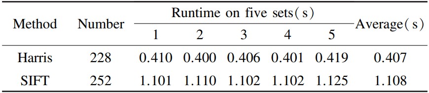
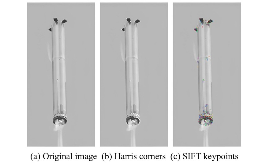
Fig.
3
Comparison of image feature detection: Original image, Harris corner detection, and SIFT keypoints
In contrast, SIFT offers higher feature uniqueness and accuracy but suffers from higher computational complexity and longer runtime. By improving the Harris method, we can retain its efficiency while enhancing accuracy and reducing false detections. This makes the improved method ideal for applications like rocket booster recovery, where both accuracy and real-time performance are essential. The enhanced approach effectively balances rapid computation with detection accuracy for efficient and precise feature extraction.
The traditional Harris algorithm detects more feature points in all test images than the improved ARH method. However, many of these points are redundant, which decreases overall accuracy(Fig.4). In contrast, the ARH algorithm detects slightly fewer points while minimizing redundancy, thereby enhancing feature extraction.
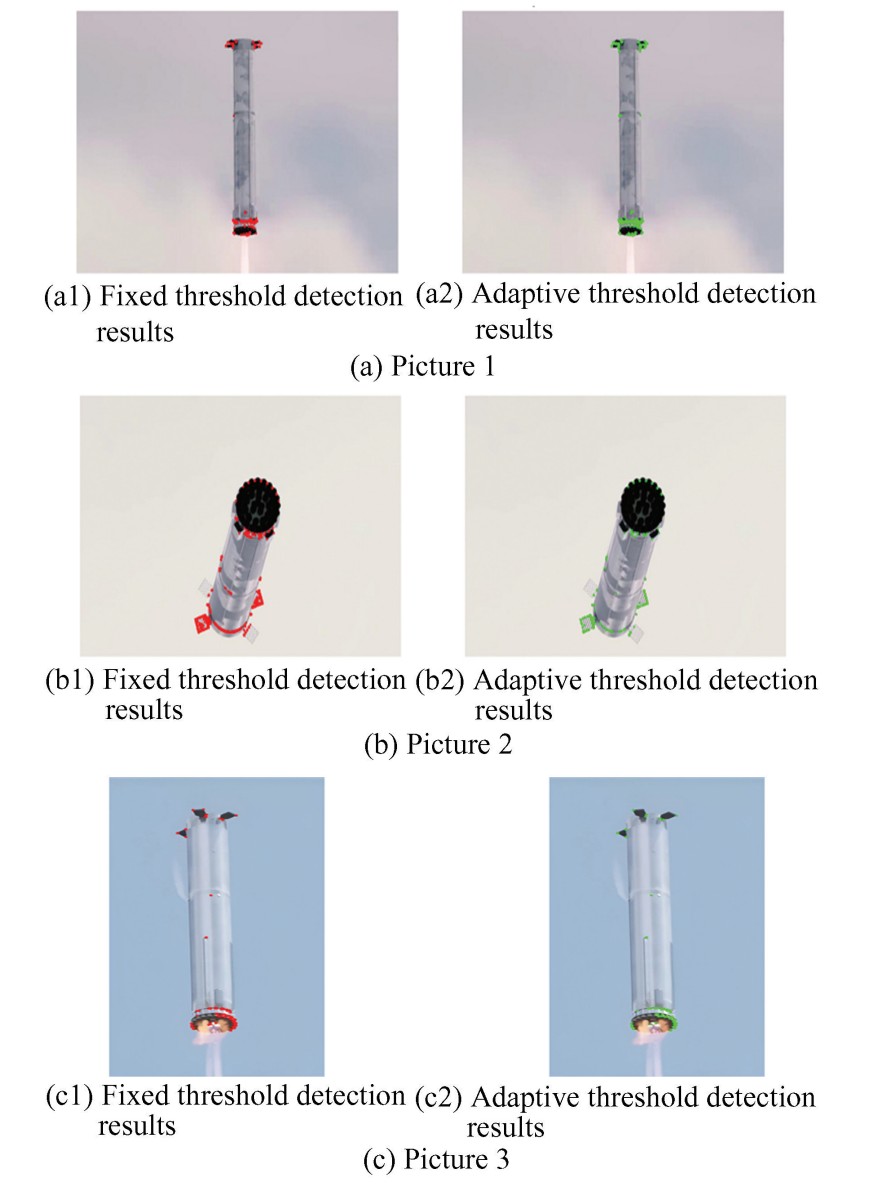
Fig.
4
Comparison of fixed threshold and adaptive threshold detection results
The ARH method is also significantly more efficient, with shorter runtimes, making it better suited for rapid-response scenarios. It maintains detection quality while reducing processing time, ideal for real-time applications.
While the traditional Harris algorithm requires complex manual threshold adjustments, the improved algorithm employs adaptive thresholding for automatic adjustments based on image content, reducing tuning time and improving efficiency.
In terms of computational efficiency, the improved algorithm without NMS is about 50% more efficient than the traditional version(Table 2). Fig.5 provides a direct representation of the data. However, false corner detection persisted. The improved algorithm with NMS effectively reduces false corners while maintaining efficient feature extraction, balancing both efficiency and accuracy, making it suitable for applications that require both real-time performance and precision.
Table
2
Without NMS:comparison between ARH and traditional Harris
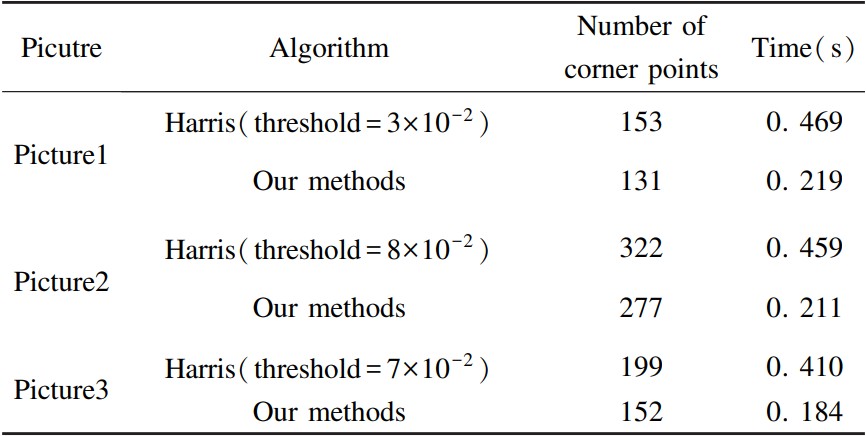
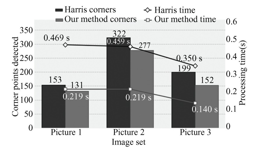
Fig.
5
Comparative analysis of corner detection performance: Harris operator vs. proposed method
2) Robustness in noisy environments.
During the recovery of rocket boosters, Gaussian noise is a major factor affecting image quality and feature detection accuracy(Fig.6). High-speed flight and extreme environmental conditions, such as vibrations, flames, and smoke, make sensors vulnerable to thermal noise and electronic interference, resulting in Gaussian noise. This random noise can lead to numerous false corners and incorrect detections, thereby impacting the accuracy and robustness of critical operations such as attitude adjustment and precise landing.
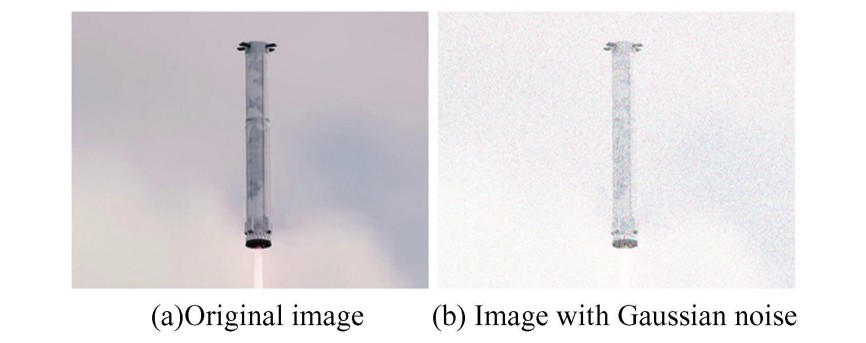
Fig.
6
Comparison before and after Gaussian noise
To mitigate the effects of Gaussian noise, filtering techniques such as Gaussian or median filtering are often employed alongside improved feature extraction algorithms, adaptive thresholding, and NMS to enhance the stability and accuracy of feature point detection.
Fig.7 compares ARH, Harris, ORB and SIFT under Gaussian noise levels 𝜎=10-50. As 𝜎 increases, ARH's repeatability gently decreases from 0.98 to 0.72—its overall average remaining above 0.85—whereas Harris falls sharply to 0.52 and ORB/SIFT drops to 0.59 and 0.72, respectively. All four methods show a slight initial rise in detected corner count, followed by a gradual decline as noise intensifies. In terms of localization accuracy, ARH keeps its mean displacement below 2.7 px, while Harris, ORB, and SIFT exhibit larger shifts of up to 4.7 px, 4.5 px, and 4.4 px, respectively. Computationally, ARH matches ORB in runtime, both affording high efficiency suitable for real-time use. Overall, ARH more consistently extracts structurally meaningful and spatially reliable keypoints in high-noise environments, thereby providing robust support for visual tracking in rocket booster recovery.
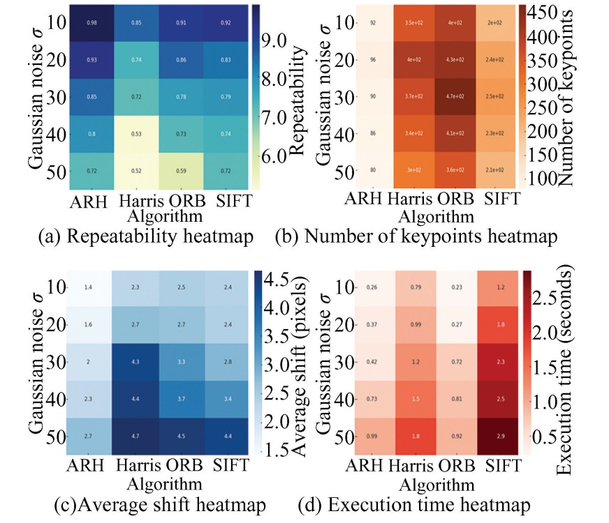
Fig.
7
Heatmap comparison of algorithm performance under different levels of Gaussian noise
3) Performance in environments with motion blur and occlusion.
a) The descent of rocket boosters at high speeds(>300 m/s) presents significant challenges for imaging systems due to rapid motion and complex environmental factors. The motion blur primarily results from two sources: 1) Linear motion blur, caused by the high-speed linear movement of the booster, manifesting as smearing along the direction of motion; 2) Random jitter blur, induced by engine vibrations and atmospheric turbulence, leading to high-frequency pixel-level displacements. To simulate these effects, a linear blur filter with a kernel size of 15 was used. The high-speed motion-induced blur obscures feature points and reduces detection accuracy, while random jitter destabilizes image capture, further complicating the matching of feature points between frames. The performance of four algorithms—improved algorithm, Harris, SIFT, and ORB—was evaluated under these conditions, as shown in Fig.8.
b) Environmental factors during landing, such as smoke, dust, and variable lighting, significantly impact image quality. Smoke and dust obstruct the camera's view, particularly under low visibility conditions at night, which are simulated using a semi-transparent texture overlay(intensity parameter=0.5 corresponding to 50% transmittance). Changing lighting conditions due to altitude and cloud cover during flight alter brightness and contrast, complicating consistent feature recognition. These effects are simulated using Gaussian noise generation(𝜎=50) and 21×21 Gaussian blur(𝜎=10) to replicate smoke diffusion, as demonstrated in Fig.9.
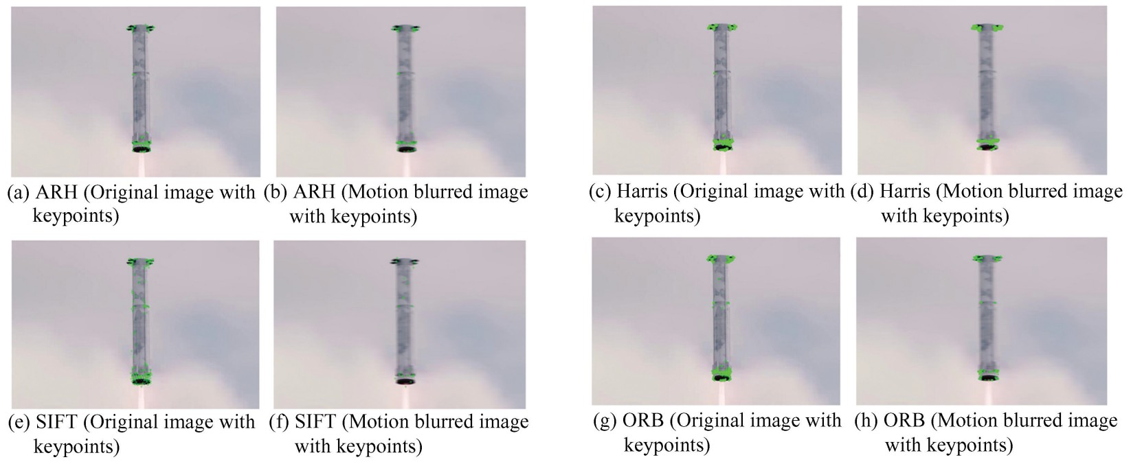
Fig.
8
Comparison of keypoint detection by different algorithms on original and motion-blurred images
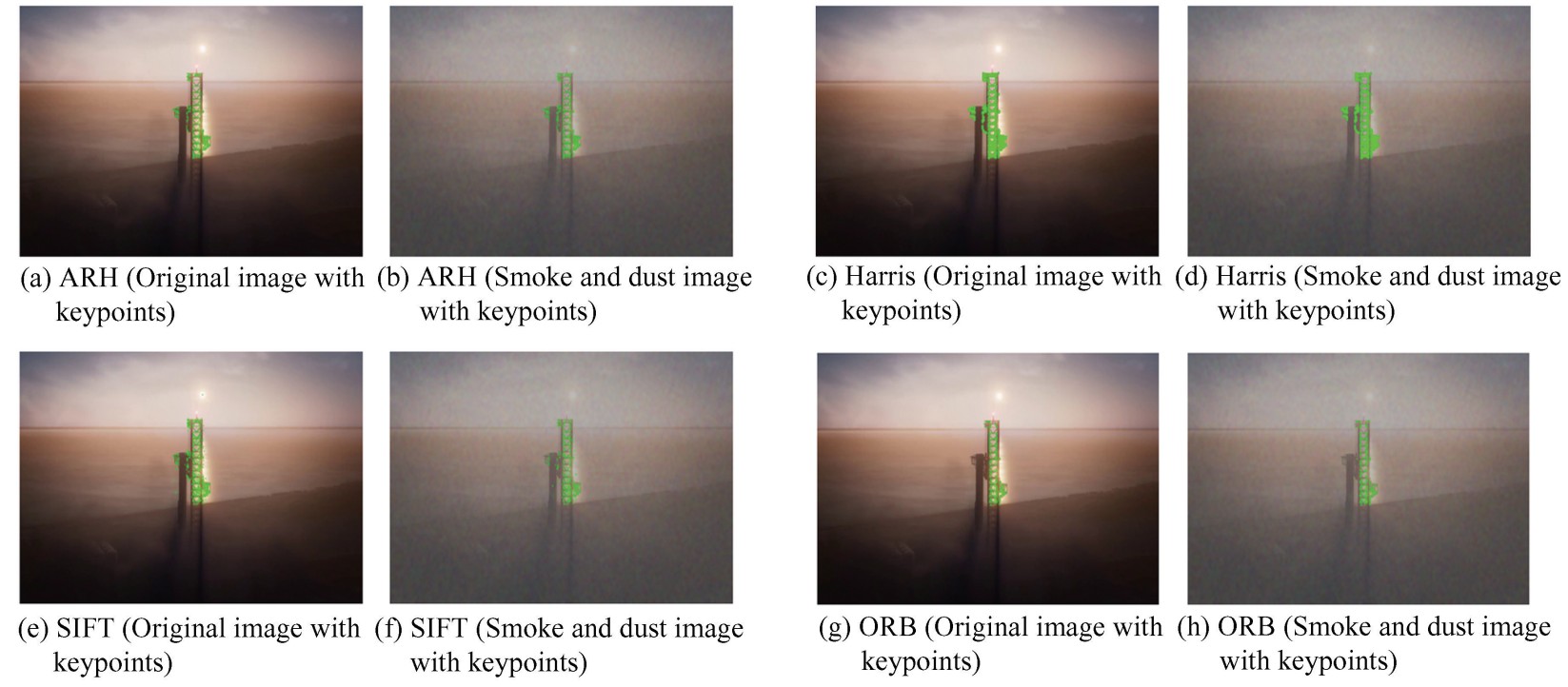
Fig.
9
Comparative analysis of keypoint detection for different algorithms under original and smoke-and-dust disturbed image conditions
c) During rocket recovery, lens contamination from oil or water droplets presents significant challenges. These contaminants substantially degrade image quality, simulated in this study through randomly generated opaque spots(density 50, max radius 30 pixels) that obscure essential feature points. The spatial randomness of these spots is ensured by their completely random distribution, preventing any patterned artifacts. Additionally, the size diversity of the spots, with radii randomly varying between 5 and 30 pixels, simulates contaminants of different particle sizes. The optical scattering effect is modeled using medium gray tones(100-200), which balance absorption and reflection effects. Such contamination compromises the accuracy and stability of feature extraction(causing an average 35% loss of feature points and a 0.4-pixel increase in displacement error), thereby affecting precise positioning and control during recovery operations. The comparative performance of algorithms under these conditions is shown in Fig.10. These challenges underscore the critical need for feature detection algorithms to maintain robust in extremely complex environments to enable effective rocket booster imaging and control.
Table 3 presents a performance comparison of various corner detection algorithms under different disturbance conditions, including blur, lens dirt, and smoke and dust occlusion. The table provides key performance metrics for each algorithm, including the number of original and processed keypoints, keypoint ratio, repeatability, average offset, execution time, and a special metric for corner reduction. Figs.11, 12, and 13 visually illustrate the metrics for each algorithm across the three different scenarios.
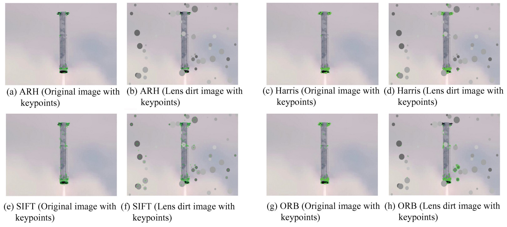
Fig.
10
Detailed comparison of keypoint detection performance for different algorithms under original and lens dirt interference conditions
Table
3
Performance comparison of corner detection algorithms under various disturbance conditions
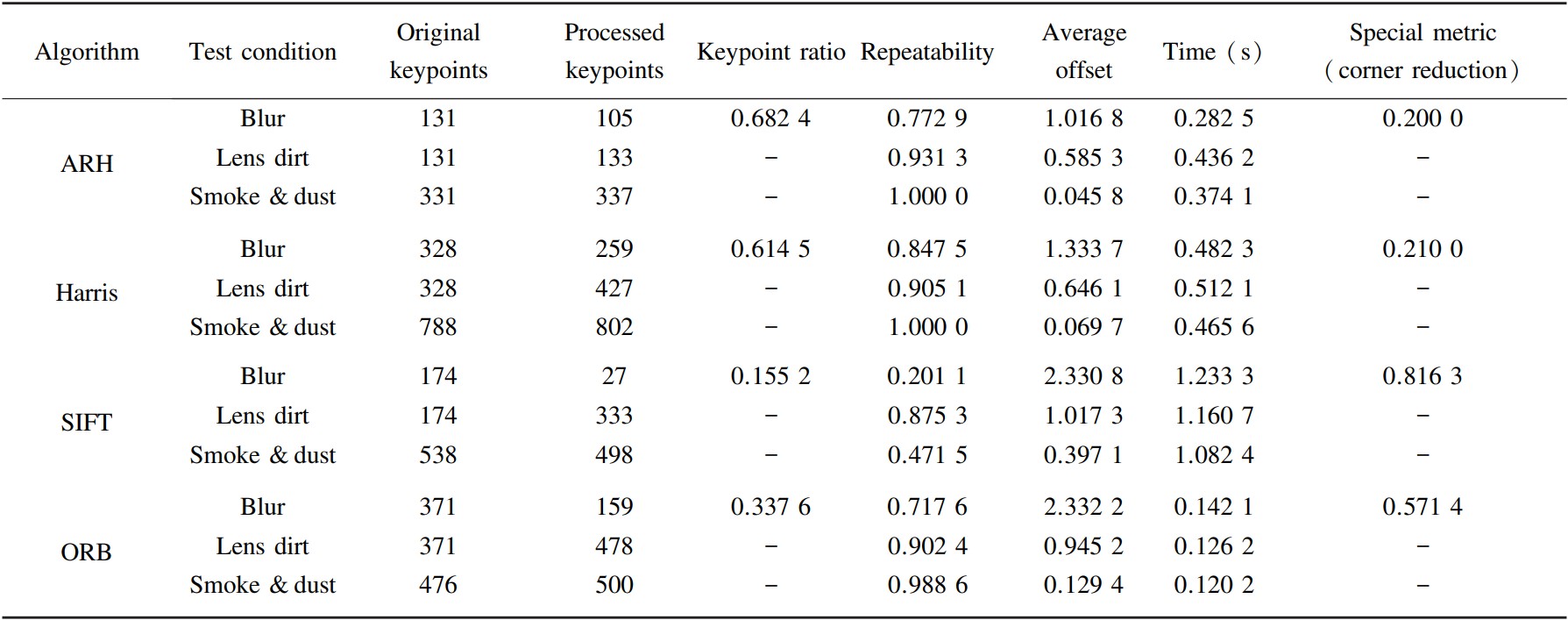
In scenarios involving motion blur, the improved ARH algorithm demonstrates excellent performance across multiple metrics(Fig.11). The ARH algorithm achieves the lowest feature point reduction rate of 20%, with a repeatability score of 0.772 9, indicating strong feature retention and robustness to motion blur. Moreover, its computation time is only 0.282 5 s, second only to ORB, providing high real-time performance. The traditional Harris algorithm detects the most feature points in the original image(328 points), many of which are redundant feature points and corner clusters. While it maintains the highest repeatability under motion blur(0.847 5), its computation time is longer(0.482 3 s), resulting in slightly lower real-time performance. The SIFT algorithm experiences a significant reduction in feature points(81.63%) under motion blur, reflecting its high sensitivity to blur. Its computation time is the longest, at 1.233 3 s, which limits its applicability in such scenarios. In contrast, while ORB excels in computational efficiency(0.142 1 s), it shows a higher feature point reduction rate of 57.14% and a repeatability score of 0.717 6, indicating its high sensitivity to blur. Overall, the improved ARH algorithm outperforms the others in terms of resistance to blur, feature point reduction, detection accuracy, and computational efficiency, making it particularly suitable for handling blur variations in high-speed moving objects such as rockets.
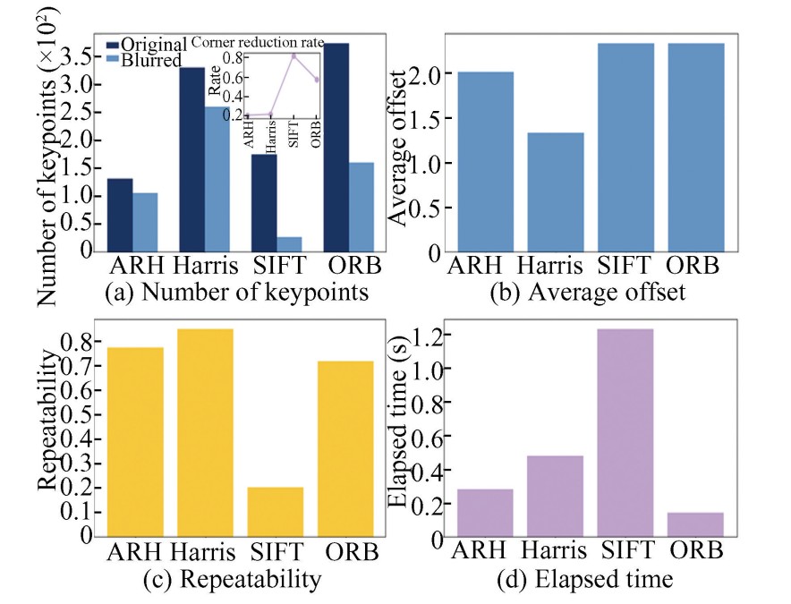
Fig.
11
Detailed comparative analysis of keypoint detection performance for different algorithms under blurred conditions: Number of keypoints, repeatability, average shift, and execution time
In smoke and dust occlusion conditions, the ARH algorithm performs excellently(Fig.12). It strikes an effective balance between repeatability, robustness, localization accuracy, and computational efficiency.The algorithm demonstrates high repeatability(1.0) in occluded environments, ensuring stable feature point detection despite environmental changes. It maintains a nearly consistent number of detected points under smoke and dust conditions, showing strong adaptability in low-contrast scenarios. Furthermore, the average displacement of detected feature points is minimal(0.045 8 pixels), indicating high localization precision, which is crucial for accurate matching. Although its execution time(0.374 1 s) is slightly longer than ORB's, the ARH algorithm provides a good trade-off between accuracy and efficiency, ensuring real-time performance. Overall, the ARH algorithm offers significant advantages in repeatability, localization accuracy, and computational efficiency, making it particularly well-suited for visual recognition and navigation in complex environments.
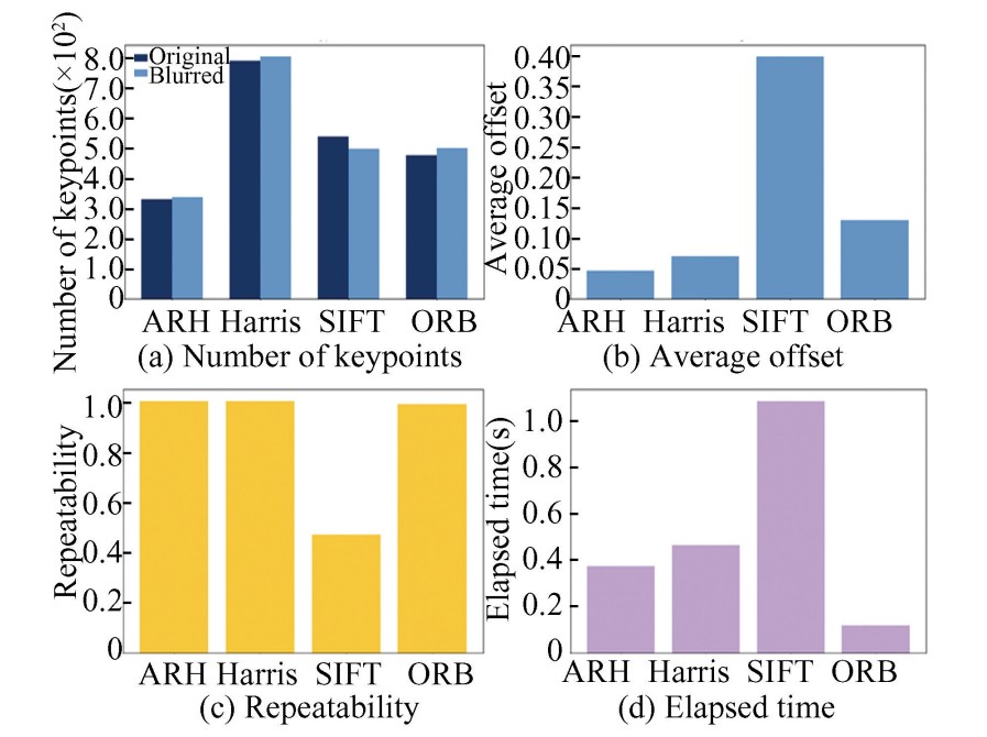
Fig.
12
Detailed comparative analysis of keypoint detection performance for different algorithms under realistic smoke and dust conditions: Number of keypoints, repeatability, average shift, and execution time
In simulated lens stain occlusion conditions, key evaluation metrics include repeatability, the number of feature points(in both original and occluded images), average displacement, and execution time(Fig.13). While the traditional Harris algorithm achieves relatively high repeatability(0.905), it suffers from a considerable number of false detections under interference, and excessive corner clustering further compromises detection precision.In contrast, the improved ARH algorithm achieves a superior balance between efficiency and robustness. It demonstrates higher repeatability(0.931) than the traditional Harris, and maintains a stable number of feature points under occlusion(ranging from 131 to 133), indicating strong adaptability to complex conditions. Furthermore, it achieves a moderate average displacement(0.585 pixels) with a substantially reduced execution time(0.436 2 s), making it highly suitable for applications requiring both real-time performance and robustness.The SIFT algorithm identifies a large number of feature points under unobstructed conditions(174 points); however, it is prone to numerous false detections when lens stains are present, resulting in a high average displacement(1.01 7 pixels). Although SIFT is well-suited for environments demanding high localization accuracy, its significantly longer processing time renders it unsuitable for real-time applications.The ORB algorithm exhibits the shortest execution time(0.126 2 s), offering excellent real-time performance and fewer false detections under occlusion. Nevertheless, it still suffers from occasional erroneous detections, which limits its applicability in highly complex environments.
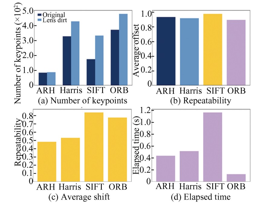
Fig.
13
Detailed comparative analysis of keypoint detection performance for different algorithms under original and lens dirt interference conditions: number of keypoints, repeatability, average shift, and execution time
In conclusion, the ARH algorithm performs excellently under various challenging conditions, including motion blur, smoke and dust occlusion, and lens stain occlusion. It strikes the optimal balance between accuracy, repeatability, localization precision, and computational efficiency, making it highly suitable for real-time applications in dynamic environments, such as visual recognition and navigation in rocket booster recovery. While the traditional Harris algorithm and SIFT offer high repeatability, their low computational efficiency or sensitivity to blur limit their applicability in real-time scenarios. ORB excels in computational efficiency but sacrifices feature detection accuracy and robustness. Overall, the ARH algorithm stands out for its ability to handle complex environmental variations, providing a robust solution for high-speed, high-precision tasks, making it suitable for real-time applications in real-world scenarios.
2.4 Other Evaluation Metrics
1) Rotational invariance.
During the rocket booster recovery process, the attitude control subsystem needs to precisely control the heading angle, especially during the approach phase(within a 300 m range). The booster's rotation around the longitudinal axis(0°-180°) causes changes in the imaging perspective, which directly affect the spatial coordinates of feature points. To evaluate the robustness of the algorithm under rotational environments, we simulate different rotational postures through geometric transformations. The image rotation angles(𝜃) range from 0° to 180° to simulate the booster's rotation process, influencing the feature point detection capability of the visual system.
When the image is rotated by an angle 𝜃, the transformation of the gradient is given by:
(21a)
(21b)
where 𝐼𝑥 and 𝐼𝑦 represent the gradients of the image in 𝑥 and 𝑦 directions respectively, and are the rotated gradients.
After rotating the gradient, we obtain the new Harris matrix 𝑴.
(22)
The rotated Harris matrix is:
(23)
where 𝑹(𝜃) is the rotation matrix. Since the determinant and trace of 𝑴 remain invariant under similar transformations, the Harris response 𝑹 also remains unchanged. Combined with the aforementioned improvements, this enhances the robustness of the detector under image rotations.
2) Comparative verification experiment.
A systematic evaluation of the performance of four feature detection algorithms with respect to image rotational invariance was conducted. The repeatability and variation in the number of keypoints under different rotation angles were examined for each algorithm. By analyzing the experimental data, we gain a more comprehensive understanding of each algorithm's feature extraction capability and stability in rotational scenarios. The algorithms evaluated include ARH, ORB, Harris, and SIFT.
(1) Repeatability evaluation.
The ARH and ORB algorithms exhibited high repeatability, nearing 1.0 across rotation angles(Fig.14), demonstrating strong feature consistency and rotational invariance. In contrast, the Harris algorithm showed significant fluctuations at specific angles(e.g., 45° and 135°), indicating poor consistency and greater sensitivity to rotation. The SIFT algorithm maintained relatively stable repeatability but experienced notable drops at some angles.
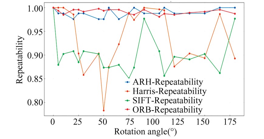
Fig.
14
Rotation invariance evaluation for different algorithms: repeatability vs. rotation angle
(2) Keypoint quantity evaluation.
The Harris algorithm displayed considerable variation in keypoint quantity, with sharp decreases at 45° and 175°, undermining reliability. The ORB algorithm maintained about 400 keypoints throughout rotation, showcasing good stability. The ARH algorithm sustained around 200 keypoints with some fluctuations, outperforming traditional Harris. SIFT showed limited variations, maintaining about 100 keypoints, indicating stability but restricting its applicability(Fig.15).
(3) Comprehensive evaluation.
Rotational invariance: ARH and ORB significantly outperformed others in repeatability, with ORB showing high consistency and excellent invariance. ARH also approached 1.0, indicating strong matching reliability.
Keypoint quantity stability: The Harris algorithm's fluctuations negatively impacted feature extraction quality, while ORB and SIFT maintained stability, with ORB excelling in consistent keypoint distribution. ARH showed some fluctuation but overall superior performance compared to Harris.
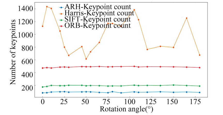
Fig.
15
Keypoint count comparison for different algorithms at various rotation angles
Overall performance analysis: The ORB algorithm demonstrated strong stability in repeatability and keypoint quantity, making it effective for rotational invariance. Although Harris had advantages in repeatability, its unstable keypoint quantities hindered performance. SIFT's stable keypoint quantities had lower repeatability, limiting its effectiveness in rotational scenarios. The ARH algorithm, with its adaptive mechanism, offered high repeatability and stability, making it ideal for rotational transformations.
In summary, ARH and ORB excel at handling rotational changes, with ORB being the preferred choice for feature extraction due to its performance in both repeatability and keypoint quantity. ARH also demonstrates strong adaptability, making it suitable for high-consistency tasks. In contrast, Harris and SIFT have limitations in stability, necessitating careful selection for practical applications.
3 Conclusions
In conclusion, the improved Harris corner detection algorithm(ARH) proposed in this study offers significant enhancements for vision-based applications, such as rocket booster recovery. By integrating adaptive thresholding, dilation-based non-maximum suppression, and sub-pixel refinement, ARH achieves much stronger robustness against noise, motion blur, and variable lighting conditions, while maintaining high computational efficiency that meets the requirements of real-time operation. Compared with classical methods such as the standard Harris, SIFT, and ORB, ARH demonstrates superior repeatability, localization accuracy, and processing speed—making it particularly effective in challenging recovery environments featuring vibration, smoke, and dust.
However, the algorithm still has certain limitations, especially under extreme illumination changes and highly dynamic scenarios, where gradient computations may be negatively impacted. To tackle these issues and further expand the algorithm's applicability, future research will focus on incorporating deep learning-based feature representation techniques to enhance adaptability and detection accuracy in complex scenarios. Other promising research directions include multi-sensor fusion with radar or LiDAR to improve reliability, the development of better dynamic scene adaptation mechanisms, and further optimization of real-time performance on embedded platforms. These advancements are expected to broaden the application of ARH in various high-precision fields, such as visual tracking, target recognition, and autonomous navigation.
