Journal of Harbin Institute of Technology(New Series)

Design of Control Method for Pointing Control Mechanism of Large Space Flexible Antenna

doi: 10.11916/j.issn.1005-9113.24053

1. Shenyang Institute of Automation, Chinese Academy of Sciences,Shenyang 110000 ,China

2. State Key Laboratory of Robotics, Chinese Academy of Sciences,Shenyang 110000 ,China

3. University of Chinese Academy of Sciences,Beijing 101408 ,China

Funds: Sponsored by Strategic Priority Research Program on Space Science, Chinese Academy of Sciences(Grant No.XDA1502030505)

Detailed information

Corresponding author

Junlin Li, Ph.D, Professor.E-mail: lijunlin@SIA.cn.

CLC number: V443+.4,V448.2,V412.4+2,O231.2,TP273+.2

Document code: A

Article ID: 1005-9113(2025)04-0001-17

Abstract

An innovative design method is outlined in this paper for the pointing control mechanism of large space flexible antennas.This method focuses on enhancing the accuracy and stability that are crucial for large spacecraft applications, such as space solar power stations. Utilizing potential energy function analysis, the dynamics of the antenna are modeled, treating it as an equivalent n-joint robotic arm. This approach simulates the rigid-flexible coupling effect through joint angle manipulations. The proposed HJI(Hamilton-Jacobi-Inequality) sliding mode robust control integrates HJI principle, dissipative system theory, and sliding mode control, offering improved pointing accuracy and robustness. Simulation results underscore the superiority of HJI sliding mode robust control over traditional PD(proportional-derivative) control in initial response, precision, and control smoothness, albeit at the cost of higher control torque requirements. This research underscores the potential of HJI sliding mode robust control in facilitating precise pointing control for future large space structures, enabling efficient space missions and reliable energy transmission.

Keywords

large flexible antennas / ground-pointing control / strong nonlinearity / sliding mode robust control / Hamilton-Jacobi inequality

0 Introduction 1 Application Scenario and Feasibility Analysis 1.1 Space Large Flexible Antenna 1.2 Practical Significance of the Research 1.3 Equivalent Model of Antenna Control Mechanism 1.4 Feasibility Demonstration 2 Dynamic Equation 2.1 Antenna Dynamic Model 2.2 Dynamic Equation of Antenna Pointing Control Mechanism 3 Controller Design 3.1 HJI Principle and Dissipative Systems Theory 3.1.1 HJI (Hamilton-Jacobi-Inequality) principle overview 3.1.2 Dissipative systems theory 3.1.3 Relationship between dissipative systems theory and HJI principle 3.1.4 Process of assessing energy dissipation in dissipative systems theory 3.2 Control Law Design 4 Data Simulation 5 Parameter Discussion 6 Conclusions

0 Introduction

Super large spacecraft are indispensable assets for space missions and deep space exploration. One notable example is the Space Solar Power Station (SSPS) , which is envisioned to orbit the earth synchronously, efficiently converting the continuous solar radiation into electricity, as shown in Figs.1-3. This electricity is then beamed down to the earth's surface using wireless microwaves. The concept of SSPS traces its origins back to the1960s^[4]when it was first introduced by American scientist Dr. Peter. Since then, various designs have emerged from different countries, encompassing the basic abacus form, multi-rotor joints SSPS, and the innovative OMEGA SSPS.

A key element facilitating information and energy transmission between the SSPS and the ground is a gigantic flexible antenna, spanning a diameter of 1 km. Although not constructed from inherently flexible materials, this antenna exhibits flexibility due to its ultra-low fundamental frequency and an exceptionally high area-to-mass ratio. These unique properties present significant challenges to the dynamic stability and performance of the SSPS^[5].

The large flexible antenna represents a unique type of space structure, distinguished by its very low stiffness, remarkably high area-to-mass ratio, and considerable mass. Such antennas are highly susceptible to structural deformations induced by external perturbations like gravity gradients, which can negatively impact pointing accuracy. This makes their dynamic analysis distinct from that of standard spacecraft. In the realm of dynamic analysis methodologies, Wittenburg^[6] introduced the Newton-Euler method, a representative vector mechanics approach widely used for analyzing large flexible structures. Another significant branch of research is analytical mechanics, where Shabana, a prominent figure, employs the Hamilton principle to model and analyze multi-flexible body systems^[7].

Fig.2Control process diagram of the design

Fig.3Schematic diagram of energy transmission to earth for a large flexible antenna^[2-3]

Over the past four decades, Kane's theorem^[8] has emerged as a novel analysis method for multibody dynamics. This theorem, building upon D'Alembert's principles, introduces deflection velocity/deflection angle velocity as an independent variable to characterize system motion. As spacecraft structures increase in size, Wie^[9] has observed a substantial decrease in structural stiffness, leading to pronounced flexibility characteristics. This flexibility can significantly impact control accuracy when the spacecraft is subjected to external interference torque.

Recent studies have extended the Udwadia-Kalaba (U-K) multi-body dynamic (MBD) formula to dynamically model flexible multibody systems using lumped parameter methods^[10]. This extension explores the natural frequencies of the system, providing deeper insights into its dynamics. Additionally, a stable and efficient cosimulation strategy has been proposed^[11], suitable for multi-flexible body dynamics (MFBD) and the discrete element method (DEM) . This integration enables the incorporation of DEM into MFBD software, enhancing the analysis capabilities for such systems.

In China, researchers have treated a flexible solar wing as a flexible beam structure^[12]. Using Lagrange equations, they established a rigid-flexible coupling primary approximate dynamic model of spacecraft. This model verifies the phenomenon of dynamic rigidity in large flexible spacecraft during rigid body motion, providing valuable insights into their behavior.

Furthermore, a finite element dynamic model has been developed for central rigid-flexible beam systems^[13-14]. This model addresses rigid-flexible coupling problems and applies classical linear quadratic regulator (LQR) technology for optimal control of central rigid-cantilever beam scenarios. This approach can be extended to other flexible spacecraft control situations, broadening its applicability and enhancing the overall control of such systems.

The quasi-sun-pointing (QSP) scheme, proposed by Li^[15] from Northwestern Polytechnical University, exhibits exceptional pointing control for large flexible structures and has the capability to track solar motion. Moreover, a proportion-differential controller has been devised to effectively minimize structural vibration amplitude, eliminating the need for attitude control torque.

Zhang's^[16] control method integrates a phase-plane controller with a high-bandwidth robust controller. This integration allows for swift antenna reorientation while reducing excessive fuel consumption caused by gravity gradient, solar light pressure, and microwave reaction torque.

Mu^[17] has developed a dual-loop control system aimed at maintaining the attitude and tracking the position of sliding masses in super-large spatial structures. To alleviate the effects of low-frequency vibrations on pointing accuracy, a vibration isolation scheme based on a quasi-zero stiffness system, consisting of computer-aided-manufacturing (CAM) , roller, and spring, has been designed.

Tanaka et al.^[18] introduced an intelligent reflector antenna system. It features a deformable secondary reflector and six actuators that work in conjunction with the main reflector. This system compensates for the impact of main reflector deformation on pointing accuracy.

Andrea and Mclnnes^[19] examined the scaling rule of attitude actuators for orbiting solar reflectors. This rule can be applied to the pointing structure of large antennas in space-based solar power stations and solar satellites.

Angeletti et al.^[20] proposed an attitude/vibration control architecture rooted in the μ synthesis framework. This architecture addresses the decreased pointing accuracy caused by the interaction between rigid buses and flexible structures. A comparative analysis against a baseline proportional-integral-derivative (PID) controller underscores the effectiveness of robust collocated control.

Overall, these studies highlight innovative approaches to enhance pointing accuracy and control in complex and flexible space structures, paving the way for more efficient and precise space missions.

The idea of this paper is as follows: the dynamics equation of the antenna yields the target attitude, with the specific control object being the pointing control mechanism of the large flexible antenna. In this context, the pointing control mechanism of antenna is analogized to a n-joint robotic arm by utilizing potential energy function analysis, and its attitude control is achieved through the manipulation of the robotic arm's joint angle changes.

1 Application Scenario and Feasibility Analysis

1.1 Space Large Flexible Antenna

Space solar power stations convert solar energy into electricity via solar panels and transmit the energy back to earth wirelessly, such as microwaves or laser beams. In this process, space large flexible antenna plays a crucial role. They can not only serve as receiving antennas, effectively capturing microwave or laser beams from space, but also serve as transmitting antennas, wirelessly transmitting electrical energy to ground receiving stations in a stable and efficient manner. This wireless transmission method overcomes the limitations of traditional cable transmission and improves the flexibility and coverage of energy transmission.

1.2 Practical Significance of the Research

In the “Guidance for the First Batch of Major Projects of the 14th Five-Year Plan” released by the National Natural Science Foundation of China (NSFC) in 2021, a project concerning “Space Assembly Dynamics and Control of Ultra-Large Aerospace Structures” was highlighted, with a pressing issue identified as the complex coupling problems in such structures. In line with this, the “Zhuri Project” (literally translating to “Chasing the Sun Project”) , aiming to establish a gigawatt (GW) -scale space solar power station by 2050, underscores the importance of addressing these challenges.

Furthermore, the “Tiangong Kaiwu Initiative”, proposed at the First Space Science and Experimental Academic Exchange Conference of the Chinese Society of Astronautics in September 2023, which envisions visioning the capability for resource exploration and development throughout the Solar System by 2100, underscores an even more urgent need for ultra-large aerospace structures, particularly large flexible antennas capable of wireless energy transmission. Pursuing research in this area can help China secure a leading position in future space exploration and development endeavors, while also fostering short-term advancements in large commercial satellites and space stations expansion.

By delving into the dynamics and control of these intricate structures, China stands poised to not only contribute significantly to the global space science landscape but also facilitate economic growth and technological innovation through the development of large-scale space-based infrastructure.

1.3 Equivalent Model of Antenna Control Mechanism

In this paper, the large flexible antenna of multi-rotating joint space solar power station (MRSSPS) proposed by Hou^[21], Qian Xuesen Space Technology Laboratory of China Academy of Space Technology, is taken as the research object.

As shown in Fig.4, the attitude control mechanism of MRSSPS is connected to other parts through a very long truss structure, and the analysis of the antenna attitude control mechanism can be regarded as the analysis of an ultra-long rod structure (attitude control mechanism + truss) ^[5]. Due to the interference from the space environment, the structure will deform and the accuracy of the antenna to the ground will be reduced. Therefore, it is necessary to restrain the deformation of the combined “bar structure” in the design control method.As shown in Fig.5, when the spacecraft is motivated to deform in orbit (Synchronous earth orbit) , it is mainly perpendicular deformation, so the paper mainly studies the perpendicular deformation of the structure.In Fig.5, L is the length of the spatial structure.

Fig.4Schematic diagram of MRSSPS

Fig.5Structure shape variable diagram of space rod under different lengths

This paper employs the potential energy function analysis method to establish an equivalent dynamic equation, which treats an ultra-long rod-like structure as an equivalent n-joint robotic arm, as shown in Fig.6. The deformation of the structure is simulated by the rotation of each segment around its corresponding joint, with larger joint angles indicating more pronounced deformation. The overall deformation of the structure is reflected by the total potential energy function, which is calculated as the weighted sum of individual potential energy functions. The weight coefficients of these individual potential energy functions in the equivalent model are determined by the deformation magnitudes observed at different locations in the actual spatial rod-like structure.

Fig.6Schematic diagram of equivalent dynamics model of very large space structure

1.4 Feasibility Demonstration

The potential energy function method is widely used in the field of spacecraft control. For example, the potential energy controller designed based on the artificial potential function method can effectively guide the spacecraft to avoid obstacles and accurately dock the target spacecraft in the close rendezvous and docking missions. In addition, in spacecraft attitude redirection control, the potential energy function method is also used to solve the attitude planning problem under multiple constraints.The equivalent dynamic model of aerospace structure is established by using this method. The following outlines the main aspects of feasibility analysis:

1) Theoretical foundation.

Potential energy function: A potential energy function is used to describe the energy of an object in different positions or states. For a system like an elastic rod, its potential energy mainly comes from elastic deformation. By accurately describing the potential energy function of the elastic rod, we can capture the key characteristics of its dynamic behavior.

2) Lagrange equations.

The Lagrange equations are a powerful tool for describing the dynamics of systems. They establish the motion equations of a system through the difference between its kinetic and potential energies (i.e., the Lagrange function) . This method is particularly suitable for complex multi-degree-of-freedom systems, such as multi-joint robotic arms.

3) Equivalent modeling.

Similarity between elastic rods and robotic arms: When subjected to force, elastic rods undergo bending deformation, and their dynamic behavior can be analogized to the coordinated motion of various joints in a multi-joint robotic arm. By reasonably dividing the elastic rod and equating each segment to a lightweight connecting rod, assuming these rods are connected by hinges, we can establish an approximate multi-joint robotic arm model.

4) Degrees of freedom and generalized.

(1) Coordinates. After equating the elastic rod to a multi-joint robotic arm, the angle of each joint can serve as a generalized coordinate of the system, uniquely describing the system's state. This equivalent treatment simplifies the dynamic analysis of the system.

(2) Computation and simulation. Numerical calculation: The dynamic model established using the Lagrange equations can be transformed into a series of differential equations. By solving these equations numerically, we can obtain the motion trajectory and velocity of the system under different conditions.

2 Dynamic Equation

2.1 Antenna Dynamic Model

As the primary focus of this paper is on discussing the control mechanism for antenna pointing, the dynamic modeling of the antenna itself will not be delved into in detail. Instead, we construct the position vector of the antenna within the absolute coordinate system. Leveraging the second Lagrange theorem and the Hamiltonian principle, we derive the dynamic equations for large flexible antennas. For a more comprehensive understanding of the modeling process, we recommend referring to Refs. ^[22-24].

\begin{matrix} M_{m} {\ddot{q}}_{m} + (C_{m} + G_{m}) {\dot{q}}_{m} + (K_{l} + K_{n} + \\ K_{T}) q_{m} = F \end{matrix}

(1)

where M_m is the mass matrix, C_m is the damping matrix, G_m is the additional mass matrix caused by rigid and flexible coupling, K_l is the linear stiffness matrix, K_n is the nonlinear stiffness matrix, K_T is the dynamic stiffness matrix caused by rigid and flexible coupling.q_m is the generalized coordinate for the displacement of an antenna element node.

2.2 Dynamic Equation of Antenna Pointing Control Mechanism

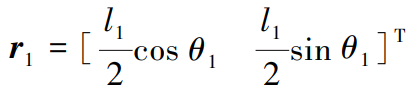
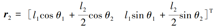
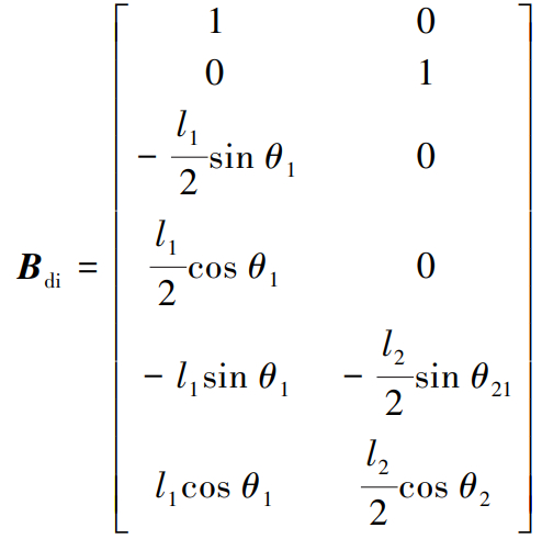
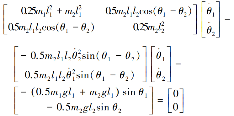
Based on the equivalent modeling theory proposed in Chapter 2 of Ref.^[25], we employ a manipulator configuration featuring two degrees of freedom to model the pointing control mechanism, Within this framework, r₁ and r₂ signify the position coordinate vectors for the two arms. Furthermore, the lengths of the robot arms are designated as l₁ and l₂, and their corresponding masses are identified as m₁ and m₂, respectively. The generalized coordinate vector, denoted as q=[θ₁ θ₂]^T, is defined to accurately describe the system configuration.

(2)

(3)

T_{1} = \frac{1}{2} m_{1} {\dot{r}}_{1}^{T} {\dot{r}}_{1} = \frac{1}{8} m_{1} l_{1}^{2} {\dot{θ}}_{1}^{2}

(4)

\begin{matrix} T_{2} = \frac{1}{2} m_{2} {\dot{r}}_{2}^{T} {\dot{r}}_{2} = \frac{1}{2} m_{2} [l_{1}^{2} {\dot{θ}}_{1}^{2} + \\ l_{1} l_{2} {\dot{θ}}_{1} {\dot{θ}}_{2} c o s (θ_{1} - θ_{2}) + \frac{l_{2}^{2}}{4} {\dot{θ}}_{2}^{2}] \end{matrix}

(5)

\frac{\partial T}{\partial θ_{1}} = \frac{\partial (T_{1} + T_{2})}{\partial θ_{1}} = - \frac{1}{2} m_{2} l_{1} l_{2} {\dot{θ}}_{1} {\dot{θ}}_{2} s i n (θ_{1} - θ_{2})

(6)

\frac{\partial T}{\partial θ_{2}} = \frac{\partial (T_{1} + T_{2})}{\partial θ_{2}} = \frac{1}{2} m_{2} l_{1} l_{2} {\dot{θ}}_{1} {\dot{θ}}_{2} s i n (θ_{1} - θ_{2})

(7)

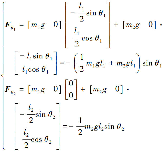
The generalized coordinate parameters θ₁ and θ₂ correspond to the generalized forces

F_{θ_{1}}

and

F_{θ_{2}}

respectively.

(8)

According to Lagrange's equation:

\frac{d}{d t} (\frac{\partial T}{\partial \dot{q}}) - \frac{\partial T}{\partial q} - F_{θ_{i}} = 0

(9)

It can be obtained:

\{\begin{matrix} [\frac{1}{4} m_{1} l_{1}^{2} {\ddot{θ}}_{1} + m_{2} l_{1}^{2} {\ddot{θ}}_{1} + \frac{1}{2} m_{2} l_{1} l_{2} {\ddot{θ}}_{2} c o s (θ_{1} - θ_{2}) - \\ \frac{1}{2} m_{2} l_{1} l_{2} {\dot{θ}}_{2} c o s ({\dot{θ}}_{1} - {\dot{θ}}_{2}) s i n (θ_{1} - θ_{2})] - \\ [\frac{1}{2} m_{2} l_{1} l_{2} {\dot{θ}}_{1} {\dot{θ}}_{2} s i n (θ_{1} - θ_{2})] - \\ [- (\frac{1}{2} m_{1} g l_{1} + m_{2} g l_{1}) s i n θ_{1}] = 0 \\ [\frac{1}{2} m_{2} l_{1} l_{2} {\ddot{θ}}_{1} c o s (θ_{1} - θ_{2}) + \frac{1}{4} m_{2} l_{2}^{2} {\ddot{θ}}_{2} - \\ \frac{1}{2} m_{2} l_{1} l_{2} {\dot{θ}}_{1} ({\dot{θ}}_{1} - {\dot{θ}}_{2}) s i n (θ_{1} - θ_{2})] - \\ [\frac{1}{2} m_{2} l_{1} l_{2} {\dot{θ}}_{1} {\dot{θ}}_{2} s i n (θ_{1} - θ_{2})] - \\ [- \frac{1}{2} m_{2} g l_{2} s i n θ_{2}] = 0 \end{matrix}

(10)

(11)

M \ddot{q} + C (q, \dot{q}) + G (q) = 0

(12)

When accounting for constraints involving nonindependent coordinates, the global coordinate vectors are established at the origin of the two segments of the manipulator arm connected to the torque actuator, as outlined below:

Since θ₁ and θ₂ are independent coordinates, the generalized coordinates can be categorized into independent and nonindependent coordinates as follows:

(13)

There exist two positions subject to position constraints: one at the articulation point between the first robotic arm and the central truss of the space power station, and the other at the articulation point between the two robotic arms. These constraints can be represented by the following two sets of equations:

\{\begin{matrix} R_{1}^{1} - \frac{l_{1}}{2} c o s θ_{1} = 0 \\ R_{1}^{2} - \frac{l_{1}}{2} s i n θ_{1} = 0 \end{matrix}

(14a)

\{\begin{matrix} R_{1}^{1} + \frac{l_{1}}{2} c o s θ_{1} = R_{2}^{1} - \frac{l_{2}}{2} c o s θ_{2} \\ R_{1}^{2} + \frac{l_{1}}{2} s i n θ_{1} = R_{2}^{2} - \frac{l_{2}}{2} s i n θ_{2} \end{matrix}

(14b)

The whole system constraint equation can be expressed as:

\begin{matrix} K (q) = [\begin{matrix} K_{1} (q) \\ K_{2} (q) \\ K_{3} (q) \\ K_{4} (q) \end{matrix}] = \\ [\begin{matrix} R_{1}^{1} - 0.5 l_{1} c o s θ_{1} \\ R_{1}^{2} - 0.5 l_{1} s i n θ_{1} \\ (R_{1}^{1} + 0.5 l_{1} c o s θ_{1}) - (R_{2}^{1} - 0.5 l_{1} c o s θ_{2}) \\ (R_{1}^{2} + 0.5 l_{1} s i n θ_{1}) - (R_{2}^{2} - 0.5 l_{1} s i n θ_{2}) \end{matrix}] = [\begin{matrix} 0 \\ 0 \\ 0 \\ 0 \end{matrix}] \end{matrix}

(15)

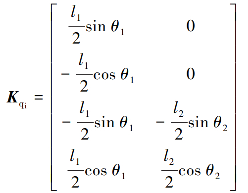
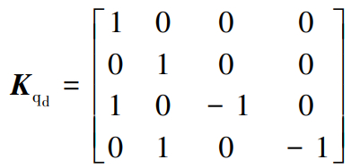
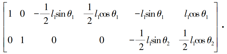
The Jacobian matrix of the entire system's constraint equation can be derived, and it can similarly be partitioned into independent coordinates and nonindependent coordinates:

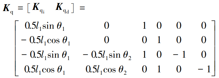
(16)

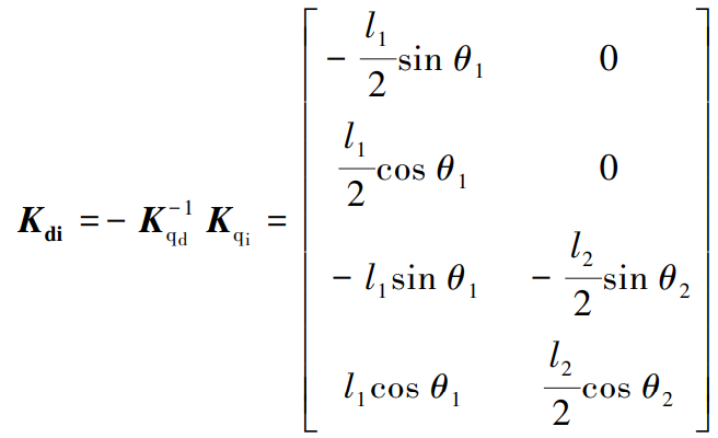
The variations of the nonindependent and independent coordinates exhibit the following relationship:

δ q_{d} = K_{d i} δ q_{i}

(17)

Hence, the generalized coordinate variation for the entire system is represented as follows:

δ q = [\begin{matrix} δ q_{i} \\ δ q_{d} \end{matrix}] = [\begin{matrix} δ q_{i} \\ K_{d i} δ q_{i} \end{matrix}] = [\begin{matrix} I \\ K_{d i} \end{matrix}] δ q_{i} = B_{d i} δ q_{i}

(18)

Due to

(19a)

(19b)

(20a)

(20b)

The kinetic energy of the system is:

T = \frac{1}{2} m_{1} {\dot{R}}_{1}^{T} {\dot{R}}_{1} + \frac{1}{2} m_{2} {\dot{R}}_{2}^{T} {\dot{R}}_{2}

(21)

The generalized inertial force vector can be obtained as follows:

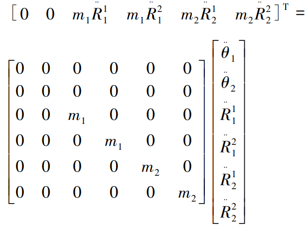
(22)

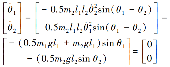
Thus, the dynamic equation of the pointing control mechanism can be derived as follows:

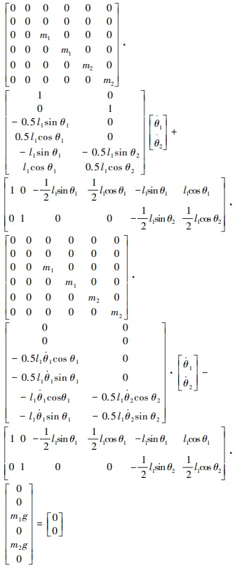
(23)

(24)

The equation is rearranged to include the first derivative of the generalized coordinates, incorporating external disturbance and modeling error terms. Given that the generalized force analyzed previously consisted primarily of heavy torque and did not account for the control torque, the control torque F is now introduced into the equation.

M (q) \ddot{q} + C (q, \dot{q}) \dot{q} + G (q) + Δ (q, \dot{q}) + d = F

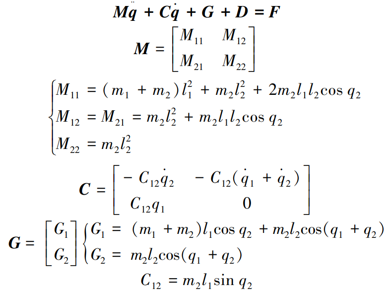
(25)

where, M (q) is the inertia matrix;

C (q, \dot{q})

is the Coriolis force term; G (q) is the gravitational term; F is the control moment;

Δ (q, \dot{q})

is the model error (caused by the model building method itself, not due to external interference) ; and d is the external inference term, which includes the gravity gradient moment, geomagnetic interference moment, light pressure moment and microwave reverse thrust moment.

Due to the extremely low fundamental frequency of large flexible antennas, they are prone to vibrations induced by excitations. In the antenna pointing control mechanism, the rigid-flexible coupling relationship between the flexible antenna and the control mechanism is reflected by the external disturbance quantity d, as well as the changes in the joint angles of the n-degree-of-freedom manipulator in the equivalent dynamic equation.

3 Controller Design

The key point of the control method designed in this paper is the combination of the HJI principle, dissipative system theorem, and sliding mode robust control. The following will explain the theoretical basis of the HJI principle and dissipative system principle used to design sliding mode robust controller, as well as the energy evaluation process, and list the design steps of the controller.The specific controller design process is shown in Fig.7.

3.1 HJI Principle and Dissipative Systems Theory

3.1.1 HJI (Hamilton-Jacobi-Inequality) principle overview

It is an inequality form based on the Hamilton-Jacobi equation, which is used to deal with optimal control, robust control and other problems. In nonlinear control systems, HJI inequalities define a partial differential inequality to solve the optimal control strategy or the control law that satisfies certain performance indexes. Compared to the standard Hamilton-Jacobi-Bellman (HJB) equation, the HJI inequality loosens the strict requirements for optimality, resulting in greater robustness when dealing with uncertainties, disturbances, or model errors.

Fig.7Controller design flow diagram

1) The theoretical basis of HJI principle is used to design controller:

(1) One of the theoretical foundations of the HJI principle lies in dynamic programming and optimal control theory. Dynamic programming provides a method for solving optimization problems with multi-stage decision processes, while optimal control seeks to find control strategies that minimize a given performance criterion. The HJB equation represents dynamic programming in continuous-time optimal control problems, and the HJI inequality is a more general form used when uncertainties or disturbances are present.

(2) Essentially, the HJI inequality is a partial differential equation (PDE) inequality. By solving this inequality, control laws that meet certain performance criteria or robustness requirements can be found. PDE theory provides mathematical tools and methods for solving the HJI inequality.

(3) Stability is a core consideration when designing controllers. The HJI inequality ensures the stability of the closed-loop system by defining a control strategy that satisfies stability conditions. By adjusting the inequality's parameters and forms, controllers with different stability and robustness characteristics can be designed.

2) Application of the HJI principle in controller design:

(1) The HJI inequality has important applications in robust controller design. By constructing appropriate HJI inequalities, control laws with strong robustness against model uncertainties, external disturbances, etc., can be derived. Such controllers maintain a certain level of performance even when system parameters change or disturbances exist.

(2) Combined with adaptive techniques such as neural networks, the HJI inequality can be used to design adaptive controllers. Neural networks can learn and identify system uncertainties online, while the HJI inequality provides a method for adjusting control strategies based on this uncertainty information. This combination enables controllers to respond and optimize control performance in real-time in dynamic environments.

(3) Although the HJI inequality relaxes strict optimality requirements, solving it can still yield near-optimal control strategies in some cases. Particularly when dealing with systems with complex dynamics and constraints, the HJI inequality provides an effective solution method.

3.1.2 Dissipative systems theory

The dissipative systems theory and the HJI principle play pivotal roles in control theory, exhibiting close connections and complementarity. The dissipative systems theory quantitatively describes the energy dissipation properties of systems through the concepts of storage functions and supply rates, while the HJI principle provides an effective tool for designing control strategies that meet specific performance criteria by solving partial differential inequalities.

3.1.3 Relationship between dissipative systems theory and HJI principle

1) Overlapping theoretical foundations.

(1) Both dissipative systems theory and the HJI principle are grounded in dynamic programming, optimal control theory, and partial differential equations (PDEs) . Dissipative systems describe the energy dissipation properties of systems through the concepts of storage functions and supply rates, whereas the HJI principle seeks to find control strategies satisfying specific performance criteria by solving partial differential inequalities.

(2) In certain cases, the inequality conditions in dissipative systems theory can be translated into HJI inequalities, particularly when considering optimal control problems for systems.

2) Design of control strategies.

(1) The dissipative systems theory provides a methodology for designing robust controllers by ensuring the system's dissipativity with respect to a given supply rate, thereby achieving robustness against uncertainties and disturbances.

(2) Similarly, the HJI principle is utilized for designing optimal or suboptimal control strategies, particularly in the presence of uncertainties or disturbances. Solving HJI inequalities yields control laws that meet specified performance criteria.

3) Stability analysis.

(1) The storage function and supply rate concepts in dissipative systems theory are intimately related to Lyapunov stability theory, facilitating the analysis of system stability.

(2) When designing control strategies using the HJI principle, the impact of the control strategy on system stability is often considered to ensure that the closed-loop system satisfies stability conditions.

3.1.4 Process of assessing energy dissipation in dissipative systems theory

1) Definition of storage function and supply rate.

(1) For a dissipative system, a non-negative storage function S (x) must first be defined, representing the “stored energy” of the system at state x.

(2) Additionally, a supply rate function s (u, y) is defined, which quantifies the “supplied energy” to the system from external inputs u and outputs y.

2) Establishment of dissipation inequality.

(1) The dissipation inequality characterizes the energy dissipation behavior of the system over any time interval [t₀, t₁], stating that the stored energy at time t₁ is no greater than the stored energy at time t₀ plus the supplied energy over that interval.

(2) Mathematically, this is expressed as:

S (x (t_{1})) ⩽ S (x (t_{0})) + \int_{t_{0}}^{t_{1}} S (u (τ), y (τ)) d τ

3) Analysis of system dissipativity:

(1) The dissipativity of the system is assessed by verifying whether the dissipation inequality holds for all admissible input functions and initial conditions. If the inequality holds for all such cases, the system is deemed dissipative.

(2) If the dissipation inequality holds with equality, the system is conservative. Furthermore, if the storage function is not restricted to being non-negative, the system is called cyclically dissipative.

4) Application of dissipativity in controller design.

(1) In controller design, the properties of dissipative systems can be leveraged to develop control strategies that meet specific performance requirements. For instance, by appropriately selecting the supply rate function and storage function, robust controllers can be designed that are resilient to uncertainties and disturbances.

(2) Moreover, dissipativity can be employed to analyze system stability and the interconnection stability of different systems.

Based on the above, the HJI sliding mode robust controller is designed using the HJI principle and dissipative system theory. The following are the specific design steps.

3.2 Control Law Design

For nonlinear systems

\sum : \{\begin{matrix} \dot{x} = f (x) + g (x) d, f (0) = 0 \\ y = h (x), h (0) = 0 \end{matrix}

(26)

If it is dissipative with respect to the supply rate

s (d, y) = \frac{1}{2} γ^{2} ‖ d ‖^{2} - \frac{1}{2} ‖ y ‖^{2}

, the L₂-gain (we define it as J) ≤γ, there exists a storage function S: χ→R⁺:

\begin{matrix} S (x (t_{1})) - S (x (t_{0})) ⩽ \frac{1}{2} \int_{t_{0}}^{t_{1}} (γ^{2} ‖ d (t) ‖^{2} - \\ ‖ y (t) ‖^{2}) d t \end{matrix}

(27)

S_{x} (x) f (x, d) ⩽ \frac{1}{2} γ^{2} ‖ d ‖^{2} - \frac{1}{2} ‖ h (x, d) ‖^{2}, \forall x, d

(28)

Note:The supply rate represents the rate at which the system receives energy from external inputs. In control theory, it is usually defined as some kind of function of the input and output vectors that quantifies the amount of energy a system receives from its external environment.

The storage function represents the energy stored inside the system. It is a non-negative function that describes the level of energy stored by a system in a certain state.

In dissipative system theory, L₂-gain is an important performance index to measure the degree of energy amplification from input to output. Specifically, the L₂-gain describes the maximum upper bound on the ratio of the energy of the system's output signal to the energy of the input signal over a certain period of time.

The differential dissipation inequality (28) for ∑ amounts to:

\begin{matrix} S_{x} (x) [f (x) + g (x) d] - \frac{1}{2} γ^{2} ‖ d ‖^{2} + \\ \frac{1}{2} ‖ h (x) ‖^{2} ⩽ 0, \forall x, d \end{matrix}

(29)

A pre-Hamiltonian function K is defined by converting the dissipation inequality to a form related to the Hamiltonian function

\begin{matrix} K (x, p, u) = p^{T} f (x, u) - \\ S (u, h (x, u)) ⩽ \\ K (x, p, u^{*} (x, p)), \forall x, p, u \end{matrix}

(30)

K (x, S_{x}^{T} (x), u^{*} (x, S_{x}^{T} (x))) ⩽ 0, \forall x

(31)

If the corresponding pre-Hamiltonian operator has the largest u^* (x, p) , then the equation is as follows:

u^{*} = \frac{1}{γ^{2}} g^{T} (x) S_{x}^{T} (x)

(32)

Then the dissipation inequality is equivalent to

K (x, S_{x}^{T} (x), u^{*} (x, S_{x}^{T} (x))) ⩽ 0, \forall x

(33)

Define the Hamiltonian operator

H (x, p) = K (x, p, u^{*} (x, p))

(34)

The dissipation inequality is then further transformed into the Hamilton-Jacobi inequality:

H (x, S_{x}^{T} (x)) ⩽ 0, \forall x

(35)

\begin{matrix} S_{x} (x) f (x) + \frac{1}{2 γ^{2}} S_{x} (x) g (x) \cdot \\ g^{T} (x) S_{x}^{T} (x) + \\ \frac{1}{2} h^{T} (x) h (x) ⩽ 0, \forall x \in χ \end{matrix}

(36)

The HJI theory is described in more detail as follows ^[26-27]:

Define

J = \underset{‖ d ∣ \neq 0}{s u p} \frac{‖ h (x) ‖_{2}}{‖ d ‖_{2}} ⩽ γ

, such that

J = \underset{‖ d ∣ \neq 0}{s u p} \frac{‖ h (x) ‖_{2}}{‖ d ‖_{2}} ⩽ γ

(37)

If there exists a positive definite and differentiable function L (x) ≥0, then

\dot{L} ⩽ \frac{1}{2} \{γ^{2} ‖ d ‖_{2}^{2} - ‖ z ‖_{2}^{2}\} (\forall d)

(38)

When γ is small enough to ensure that J is small enough, and d is bounded, then there is

‖ h (x) ‖_{2} \to 0, e \to 0, \dot{e} \to 0

.It proves that the output of system y=h (x) is convergent.In summary, HJI sliding mode robust control can reduce the system error by changing the γ value, and then improve the control accuracy.

The specific steps of controller design are outlined below.The dynamic equation of the space antenna pointing control mechanism has been obtained from the Eq. (25) :

M (q) \ddot{q} + C (q, \dot{q}) \dot{q} + G (q) + Δ (q, \dot{q}) + d = F

(39)

F = u + M (q) {\ddot{q}}_{d} + C (q, \dot{q}) {\dot{q}}_{d} + G (q)

(40)

Here, u represents the feedback control law employed in HJI sliding mode robust control, while F denotes the signal corresponding to the control input. q is the actual pose information, q_d is the expected pose, and

\dot{q}

and

{\dot{q}}_{d}

are similar.The position error e and velocity error

\dot{e}

of the transmitting antenna of the space solar power station can be determined.

e = q - q_{d}, \dot{e} = \dot{q} - {\dot{q}}_{d}

(41)

The control law Eq. (40) can be substituted into the multi-body dynamics Eq. (26) to obtain the following:

M (q) \ddot{e} + C (q, \dot{q}) \dot{e} + Δ (q, \dot{q}) + d = u

(42)

Sliding mode function was defined as

s = \dot{e} + α e

, α is the error adjustment coefficient.

\{\begin{matrix} \dot{e} = s - α e \\ M \dot{s} = - C s + ω - Δ - d + u \end{matrix}

(43)

ω = M α \dot{e} + C α e, D = d + Δ

, by employing the HJI inequality, the aforementioned equation can be expressed as follows:

\{\begin{matrix} \dot{x} = [\begin{matrix} s - α e \\ \frac{1}{M} (- C s + ω + u) \end{matrix}] + [\begin{matrix} 0 \\ - \frac{1}{M} \end{matrix}] (Δ + d) \\ z = h (x) = \dot{e} + α e = s \end{matrix}

(44)

Define the positive definite and differentiable function V (x) :

V = \frac{1}{2} s^{T} M s

(45)

\begin{matrix} \dot{V} = \frac{1}{2} s^{T} \dot{M} s + s^{T} M \dot{s} = \\ s^{T} (- C s + ω - D + u) + \frac{1}{2} s^{T} \dot{M} s = \\ \frac{1}{2} s^{T} (\dot{M} - 2 C) s + s^{T} (ω - D + u) \end{matrix}

(46)

Due to the control mechanism is slanted symmetrically

\frac{1}{2} s^{T} (\dot{M} - 2 C) s = 0

(47)

Let u=-ω+k; then, Eq. (47) is equal to:

\dot{V} = - s^{T} D + s^{T} k

(48)

According to Eq. (38) , we obtain:

- s^{T} D + s^{T} k ⩽ \frac{1}{2} γ^{2} ‖ D ‖_{2}^{2} - \frac{1}{2} ‖ z ‖_{2}^{2}

(49)

When employing the aforementioned formula

s^{T} k ⩽ \frac{1}{2} γ^{2} ‖ D ‖_{2}^{2} - \frac{1}{2} ‖ z ‖_{2}^{2}

(50)

Let

k = - \frac{1}{2} s + k_{1}

. The evaluation function, z is equal to s, thus leading to the following conclusion:

- \frac{1}{2} ‖ z ‖_{2}^{2} + k_{1} s^{T} ⩽ \frac{1}{2} γ^{2} ‖ D ‖_{2}^{2} - \frac{1}{2} ‖ z ‖_{2}^{2}

So,

k_{1} s^{T} ⩽ \frac{1}{2} γ^{2} ‖ D ‖_{2}^{2}

(51)

To ensure that the above formula is established and satisfies the HJI principle, the following equation can be used:

k_{1} = - \frac{1}{2 γ^{2}} s

(52)

Because it can obtain:

- \frac{‖ z ‖_{2}^{2}}{2 γ^{2}} ⩽ \frac{γ^{2}}{2} ‖ D ‖_{2}^{2}

(53)

After the deformation of the formula, the expression for evaluating the system's anti-interference. In order to express the anti-interference performance of the system, the performance index is defined as J.

Performance index J can be derived

J = \underset{‖ d \neq 0}{s u p} ‖ \frac{‖ z ‖_{2}^{2}}{‖ D ‖_{2}^{2}} ⩾ - γ^{4}

(54)

When γ is small enough, the performance index J will be small enough, thereby enhancing the system robustness. Based on the aforementioned statement:

\begin{matrix} u = - ω + k = - ω - \frac{1}{2} s + k_{1} = \\ - ω - \frac{1}{2} s - \frac{1}{2 γ^{2}} s \end{matrix}

(55)

Due to

ω = M α \dot{e} + C α e, s = \dot{e} + α e

, we have obtained:

u = - (M α \dot{e} + C α e) - (\frac{1}{2 γ^{2}} + \frac{1}{2}) (\dot{e} + α e)

(56)

To sum up, the schematic diagram of the control system can be obtained, as shown in Fig.8.

Fig.8HJI sliding mode robust control structure diagram

The Lyapunov function is defined as follows:

L = \frac{1}{2} s^{T} M s

(57)

where M is the inertia matrix. Then, the following Eq. (58) is obtained:

\begin{matrix} \dot{L} = s^{T} M \dot{s} + \frac{1}{2} s^{T} \dot{M} s = s^{T} (- C s + ω - Δ - \\ d + u) + \frac{1}{2} s^{T} \dot{M} s = s^{T} (- d - Δ - \frac{1}{2 γ^{2}} s - \\ \frac{1}{2} s) + \frac{1}{2} s^{T} (\dot{M} - 2 C) s = - s^{T} (d + Δ) - \frac{1}{2 γ^{2}} s^{T} s - \frac{1}{2} s^{T} s \end{matrix}

(58)

Definition:

\begin{matrix} H = \dot{L} - \frac{1}{2} γ^{2} ‖ D ‖_{2}^{2} + \frac{1}{2} ‖ z ‖_{2}^{2} = \\ - s^{T} D - \frac{1}{2 γ^{2}} s^{T} s - \frac{1}{2} s^{T} s - \frac{1}{2} γ^{2} ‖ D ‖_{2}^{2} + \\ \frac{1}{2} ‖ z ‖_{2}^{2} \end{matrix}

(59)

Because of:

\{\begin{matrix} - s^{T} D - \frac{1}{2 γ^{2}} s^{T} s - \frac{1}{2} γ^{2} ‖ D ‖_{2}^{2} = - \frac{1}{2} {‖\frac{1}{γ} s + γ D‖}_{2}^{2} ⩽ 0 \\ - \frac{1}{2} s^{T} s + \frac{1}{2} ‖ z ‖_{2}^{2} = 0 \end{matrix}

(60)

Then, H≤0, the following equation can be obtained:

\dot{L} ⩽ \frac{1}{2} γ^{2} ‖ D ‖_{2}^{2} - \frac{1}{2} ‖ z ‖_{2}^{2}

(61)

According to HJI theory, J≤γ can be obtained, and the solid property index meets the requirements.

4 Data Simulation

To simplify the calculation process, the antenna control mechanism is represented as a dual-articulated mechanical arm^[28] consisting of two arms with lengths denoted as l₁ and l₂, and masses represented by m₁ and m₂, respectively. For the torque actuators installed in the space solar power station, the total length of a single robotic arm is set to 10.2 m, matching the dimensions of the robotic arm on China's Tiangong Space Station. Each segment measures 5.1 m in length, and the entire assembly weighs 370 kg, the orbital altitude is about 36000 km, the radius of the earth is about 6371 km (g≈0.222 m/s²) .

Figs.9-12 clearly shows that by increasing the error adjustment coefficient α from to 50 and 100, the system's time to achieve the desired accuracy range is significantly reduced to less than 31 s. This finding suggests that elevating the value of the error adjustment coefficient effectively enhances the system's adjustment speed. When the proportional-derivative (PD) method is employed for control (Figs.13-15) .

Fig.9HJI sliding mode robust control simulated diagram (α=50, γ=0.01)

Fig.10HJI sliding mode robust control attitude angle error simulated diagram (α=50, γ=0.01)

Fig.11HJI sliding mode robust control attitude angle error local simulated diagram (α=50, γ=0.01)

The PD control system achieves an attitude angle error accuracy of approximately 0.01°, with a steady-state time of less than 5 s. However, this level of accuracy fails to meet the stringent control accuracy requirements. The simulation diagram reveals that PD control exhibits lower control accuracy compared to HJI sliding mode robust control, and it also demonstrates an overshoot phenomenon. Nonetheless, PD control retains certain advantages in terms of convergence speed.

Fig.12HJI sliding mode robust control attitude angle error local simulated diagram (α=100, γ=0.01)

Fig.13PD control simulated diagram

Fig.14PD control simulated diagram attitude angle error diagram

Fig.15PD control attitude angle error local diagram

5 Parameter Discussion

Based on the data simulation, it is evident that the HJI sliding mode robust control achieves the desired error accuracy within 40 s (α=50, γ=0.01) .This time is further reduced to approximately 30 s when the error adjustment coefficient α is set to 100. By fine-tuning the value of α, a further decrease in convergence time can be observed from the convergence trend indicated by the simulation curve, enabling even higher accuracy conditions to be met. Although PD control demonstrates a faster convergence speed than HJI sliding mode robust control, its accuracy still falls short of the required control standards.

The following discussion delves into the influence exerted by the two control methods on attitude angle and control moment over prolonged operational periods.

As evident from Fig.16, even the anticipated attitude experiences significant vibrations during the initial phase due to uncertain interference factors. In such scenarios, without proper compensation and correction of the target attitude, despite the controller's exceptional tracking performance, the target attitude remains unstable and inaccurate. Consequently, the precise pointing control of the space antenna cannot be ensured.

Upon comparing the simulation graphs (Figs.17-20) , it becomes apparent that HJI sliding mode robust control excels in compensating for and correcting vibrations in the target attitude, particularly noticeable in the attitude angle q₂ during the initial phase. Consequently, this leads to improved control performance in subsequent tracking, ensuring greater antenna pointing accuracy for space solar power stations.

Fig.16The target attitude angle diagram under interference condition (GEO)

Fig.17HJI sliding mode robust control attitude angle variation diagram (GEO)

Fig.18PD control attitude angle variation diagram (GEO)

Taking into account various orbit factors, the orbit has been established at an altitude of 380 km, which corresponds to the orbit of China's Tiangong Space Station, where the gravitational acceleration is approximately 8.7 m/s².

Compared to simulation results obtained in geosynchronous orbit, the performance of HJI sliding mode robust control falls short of PD control in low earth orbit. Specifically, q₁ experiences periodic vibrations, indicating that the effectiveness of HJI sliding mode robust control increases with orbit altitude. This makes it highly suitable for the very large space antennas typically deployed in high orbits.

Fig.19HJI sliding mode robust control attitude angle variation diagram (LEO)

Fig.20PD control attitude angle variation diagram (LEO)

Figs.21-24 illustrate the control torque required for long-term orbit operation of a large flexible antenna using HJI sliding mode robust control and PD control, respectively. It can be observed that the maximum control torque is needed at the beginning of the control process, which gradually decreases over time. Even after the attitude of the space antenna stabilizes, a certain amount of control torque is still required to suppress vibrations and ensure antenna pointing accuracy. Notably, HJI sliding mode robust control outperforms PD control in terms of control accuracy, but it demands a higher control torque to mitigate vibrations compared to PD control.

Fig.21The torque needed of HJI sliding mode robust control (global)

Fig.22The torque needed of HJI sliding mode robust control (local)

Fig.23The torque needed of PD control (global)

In summary, HJI sliding mode robust control has significant advantages in pointing control accuracy for large flexible antennas of space solar power stations that need to operate in high orbits, such as geosynchronous orbits. In the future, it holds broad application prospects in other areas, such as attitude control of ultra-large solar sails and manned spacecraft for Mars missions.

Fig.24The torque needed of PD control (local)

6 Conclusions

Based on the potential energy function theory, this paper establishes an equivalent dynamic model for the pointing control mechanism of large flexible antennas, analogizing it to an n-joint robotic arm. The rigid-flexible coupling relationship between the rigid control structure and the flexible antenna is simulated through the rotation of joint angles.The absolute node coordinate method and the Hamilton principle are used to create a dynamic model for a large flexible antenna, pinpointing the desired attitude angle and attitude angular velocity. Through the application of the coordinate separation method, we derived the equivalent dynamic equation for the antenna pointing control mechanism, incorporating a non-independent variable constraint.The control law of HJI sliding mode robust controller is derived by HJI principle and dissipative system theorem, and its performance evaluation index is determined.When compared to traditional PD controls, the HJI sliding mode robust control demonstrates notable superiority in terms of its initial response and its ability to suppress overshoot during sine wave peak inputs for attitude signals. HJI sliding mode robust control outperforms traditional PD control in terms of pointing control accuracy and smoothness of control, but it requires a higher torque to suppress vibrations after the attitude angle changes. This indicates that HJI sliding mode robust control is particularly suitable for situations where extremely high control accuracy is demanded. In summary, while HJI sliding mode robust control excels in precision and smoothness, it comes at the cost of higher torque requirements for vibration suppression. Nonetheless, it remains an ideal choice for applications that prioritize precision control.

Acknowledgement

The authors gratefully acknowledge the support of Shenyang Institute of Automation, Chinese Academy of Sciences, and the University of Chinese Academy of Sciences.

Download: Full size image

Fig.2Control process diagram of the design

Download: Full size image

Fig.3Schematic diagram of energy transmission to earth for a large flexible antenna^[2-3]

Download: Full size image

Fig.4Schematic diagram of MRSSPS

Download: Full size image

Fig.5Structure shape variable diagram of space rod under different lengths

Download: Full size image

Fig.6Schematic diagram of equivalent dynamics model of very large space structure

Download: Full size image

Fig.7Controller design flow diagram

Download: Full size image

Fig.8HJI sliding mode robust control structure diagram

Download: Full size image

Fig.9HJI sliding mode robust control simulated diagram (α=50, γ=0.01)

Download: Full size image

Fig.10HJI sliding mode robust control attitude angle error simulated diagram (α=50, γ=0.01)

Download: Full size image

Fig.11HJI sliding mode robust control attitude angle error local simulated diagram (α=50, γ=0.01)

Download: Full size image

Fig.12HJI sliding mode robust control attitude angle error local simulated diagram (α=100, γ=0.01)

Download: Full size image

Fig.13PD control simulated diagram

Download: Full size image

Fig.14PD control simulated diagram attitude angle error diagram

Download: Full size image

Fig.15PD control attitude angle error local diagram

Download: Full size image

Fig.16The target attitude angle diagram under interference condition (GEO)

Download: Full size image

Fig.17HJI sliding mode robust control attitude angle variation diagram (GEO)

Download: Full size image

Fig.18PD control attitude angle variation diagram (GEO)

Download: Full size image

Fig.19HJI sliding mode robust control attitude angle variation diagram (LEO)

Download: Full size image

Fig.20PD control attitude angle variation diagram (LEO)

Download: Full size image

Fig.21The torque needed of HJI sliding mode robust control (global)

Download: Full size image

Fig.22The torque needed of HJI sliding mode robust control (local)

Download: Full size image

Fig.23The torque needed of PD control (global)

Download: Full size image

Fig.24The torque needed of PD control (local)

Download: Full size image

Fig.2Control process diagram of the design

Fig.3Schematic diagram of energy transmission to earth for a large flexible antenna^[2-3]

Fig.4Schematic diagram of MRSSPS

Fig.5Structure shape variable diagram of space rod under different lengths

Fig.6Schematic diagram of equivalent dynamics model of very large space structure

Fig.7Controller design flow diagram

Fig.8HJI sliding mode robust control structure diagram

Fig.9HJI sliding mode robust control simulated diagram (α=50, γ=0.01)

Fig.10HJI sliding mode robust control attitude angle error simulated diagram (α=50, γ=0.01)

Fig.11HJI sliding mode robust control attitude angle error local simulated diagram (α=50, γ=0.01)

Fig.12HJI sliding mode robust control attitude angle error local simulated diagram (α=100, γ=0.01)

Fig.13PD control simulated diagram

Fig.14PD control simulated diagram attitude angle error diagram

Fig.15PD control attitude angle error local diagram

Fig.16The target attitude angle diagram under interference condition (GEO)

Fig.17HJI sliding mode robust control attitude angle variation diagram (GEO)

Fig.18PD control attitude angle variation diagram (GEO)

Fig.19HJI sliding mode robust control attitude angle variation diagram (LEO)

Fig.20PD control attitude angle variation diagram (LEO)

Fig.21The torque needed of HJI sliding mode robust control (global)

Fig.22The torque needed of HJI sliding mode robust control (local)

Fig.23The torque needed of PD control (global)

Fig.24The torque needed of PD control (local)

Image(24)

Citation

Fuchenglong Zhao, Junlin Li.Design of control method for pointing control mechanism of large space flexible antenna. Journal of Harbin Institute of Technology(New Series),2025,32(4):1-17.

Copy

Metering

Fig.2Control process diagram of the design

Fig.3Schematic diagram of energy transmission to earth for a large flexible antenna^[2-3]

Fig.4Schematic diagram of MRSSPS

Fig.5Structure shape variable diagram of space rod under different lengths

Fig.6Schematic diagram of equivalent dynamics model of very large space structure

Fig.7Controller design flow diagram

Fig.8HJI sliding mode robust control structure diagram

Fig.9HJI sliding mode robust control simulated diagram (α=50, γ=0.01)

Fig.10HJI sliding mode robust control attitude angle error simulated diagram (α=50, γ=0.01)

Fig.11HJI sliding mode robust control attitude angle error local simulated diagram (α=50, γ=0.01)

Fig.12HJI sliding mode robust control attitude angle error local simulated diagram (α=100, γ=0.01)

Fig.13PD control simulated diagram

Fig.14PD control simulated diagram attitude angle error diagram

Fig.15PD control attitude angle error local diagram

Fig.16The target attitude angle diagram under interference condition (GEO)

Fig.17HJI sliding mode robust control attitude angle variation diagram (GEO)

Fig.18PD control attitude angle variation diagram (GEO)

Fig.19HJI sliding mode robust control attitude angle variation diagram (LEO)

Fig.20PD control attitude angle variation diagram (LEO)

Fig.21The torque needed of HJI sliding mode robust control (global)

Fig.22The torque needed of HJI sliding mode robust control (local)

Fig.23The torque needed of PD control (global)

Fig.24The torque needed of PD control (local)

Hou X B, Zhang X, Cheng Z A,et al. Concept design on modular multi-rotary joints solar power satellite. Space Electronic Technology,2023,20(3):1-6 DOI:10.3969/j.issn.1674-7135.2023.03.001.

Hou X B. Unlocking the Frontiers of Science and Technology Series: Illustrated Space Solar Power Station. Beijing: Chemical Industry Press,2023.

Tu Yiwen. The beauty of industry | China's first space solar power station experimental base under construction,“Space Three Gorges” on the way.2021. Retrieved from https://www.jiemian.com/article/6352838.html.

Peter E G. Power from the sun: Its future. Science,1968,162:867-886. DOI:10.1126/science.162.3856.857.

Hou Xinbin, Wang Li, Zhang Xinghua. Concept design on multi-rotary joints SPS. Journal of Astronautics,2015,36(11):1332-1338. DOI:10.3873/j.issn.1000-1328.2015.11.016.

Wittenburg J. Dynamics of systems of rigid bodies. Journal of Applied Mathematics and Mechanics,1979,59(7):331. DOI:10.1002/zamm.19790590712.

Shabana A A. Dynamics of Multibody Systems. Cambridge: Cambridge University Press,2005:115-123. DOI:10.1017/CBO9780511610523.

Kane T R, Levinson D A. Dynamics theory and applications. Mechanism and Machine Theory,1986,21(4):361-362. DOI:10.1016/0094-114X(86)90059-5.

Wie B, Roithmayr C. Integrated orbit,attitude,and structural control systems design for space solar power satellites. NASA Technical Memorandum,2001,210854:1-123. DOI:10.5555/888182.

Edward J H Yap, Djamel Rezgui, Mark H,et al. Modelling flexible multi-body systems within the Udwadia-Kalaba framework,a lumped parameter approach. Journal of Computational and Nonlinear Dynamics,2022,17(12):1005-1019. DOI:10.1115/1.4055957.

Sanborn G, Choi J, Choi J H. Strategy for cosimulation of multiflexible-body dynamics and the discrete element method. Journal of Mechanical Science and Technology,2021,35(10):4363-4380. DOI:10.1007/s12206-021-0908-2.

Jiang J P, Li Dongxu. Modelling and simulation for the rigid-flexible coupling dynamics of the spacecraft with flexible appendages. Journal of Astronuautics,2005,26(3):270-274.

Cai G P, Hong J Z, Yang S X. Model study and active control of a rotating flexible cantilever beam. International Journal of Mechanical Sciences,2004,46(6):871-889. DOI:10.1016/j.ijmecsci.2004.06.001.

Cai G P, Lim C W. Active control of a flexible hub-beam system using optimal tracking control method. International Journal of Mechanical Sciences,2006,48(10):1150-1162. DOI:10.1016/j.ijmecsci.2006.05.003.

Li Q J, Deng Z C, Wang Y,et al. Quasi-sun-pointing oriented attitude for solar power satellites. Journal of Astronautics 2019,1:29-40. DOI:10.3873/j.issn.1000-1328.2019.01.004.

Zhang K M. Attitude Dynamic Modelling and Robust Control of Space Solar Power Station. Dalian: Dalian University of Technology,2021:86-93.

Mu R N. Coupling Dynamic Characteristic and Attitude Control of Super Large Space Structures on Orbit. Dalian: Dalian University of Technology,2020:1-131.

Tanaka H, Kogiso N, Sakano F,et al. Experimental demonstration of deformable reflector antenna system with high accuracy deformation measurement. Acta Astronautica 2022,194:93-105. DOI:10.1016/j.actaastro.2022.02.002.

Andrea V, Mclnnes C R. Attitude control actuator scaling laws for orbiting solar reflectors. Advances in Space Research,2023,71(1):604. DOI:10.1016/j.asr.2022.10.015.

Angeletti F, Iannelli O, Gasbarri P,et al. Robust collocated control of large flexible space structures. IFAC-PapersOnLine 2022,55(25):85-90. DOI:10.1016/j.ifacol.2022.09.328.

Hou X B, Wang L, Zhang X H,et al. Concept design on multi-rotary joints SPS. Journal of Astronautics,2015,36(11):1332-1338. DOI:10.3873/j.issn.1000-1328.2015.11.016.

Shao Q, Lu Y F, Shi C,et al. Rigid-flexible coupled nonlinear dynamics and analysis of space membrane structure. Chinese Space Science and Technology,2022,42(1):47-56. DOI:10.16708/j.cnki.1000-758X.2022.0005.

Li M G, Qian L. Dynamical System Modelling and Simulation.2th ed. Beijing: National Defense industry Press,2015.10-103.

Teodorescu P P. Mechanical Systems, Classical Models: Volume III: Analytical Mechanics. Heidelberg: Springer 2009:1-351.

Du W Z, Yao X G, Cao D Z. Fundamentals of Dynamics of Multibody Systems. Beijing: Beijing University of Aeronautics and Astronautics Press,2021:1-100.

Colombo R M, Perrollaz V, Sylla A. Conservation laws and Hamilton-Jacobi equations with space inhomogeneity. Journal of Evolution Equations 2023,23(3):1-72. DOI:10.1007/s00028-023-00902-1.

Kalise D, Kunisch K. Hamilton-Jacobi-Bellman Equations: Numerical Methods and Applications in Optimal Control. Berlin: De Gruyter,2018:1-50.

Liu J K. Sliding Mode Control Design and MATLAB Simulation the Basic Theory and Design Method.4th ed. Beijing: Tsinghua University Press,2019:79-149.

0 Introduction

1 Application Scenario and Feasibility Analysis

2 Dynamic Equation

3 Controller Design

4 Data Simulation

5 Parameter Discussion

6 Conclusions

LINKS